Validating Materials Characterization Techniques: A Guide for Robust Biomedical Research and Drug Development
This article provides a comprehensive framework for the validation of materials characterization techniques, a critical process for ensuring data reliability in biomedical research and drug development.
Validating Materials Characterization Techniques: A Guide for Robust Biomedical Research and Drug Development
Abstract
This article provides a comprehensive framework for the validation of materials characterization techniques, a critical process for ensuring data reliability in biomedical research and drug development. It covers foundational principles, from defining Certified Reference Materials (CRMs) and metrological traceability to the SI units, to the application of novel methodologies and standards for complex materials like nanomaterials and advanced alloys. The content further addresses common troubleshooting scenarios, offers strategies for optimizing measurement efficiency, and outlines rigorous procedures for method validation and comparative analysis. Designed for researchers, scientists, and drug development professionals, this guide synthesizes current best practices and emerging trends to empower teams in navigating regulatory challenges and enhancing the quality and impact of their characterization data.
The Pillars of Validation: Principles, Reference Materials, and Traceability
Understanding Certified Reference Materials (CRMs) and Reference Test Materials (RTMs)
In the scientific disciplines of chemistry, materials science, and pharmaceutical development, the validity of research and the reliability of industrial quality control hinge on the accuracy and comparability of measurements. Reference Materials (RMs), Certified Reference Materials (CRMs), and Reference Test Materials (RTMs) constitute the fundamental metrological tools that underpin this framework. These materials are essential for calibrating instruments, validating methods, and ensuring traceability to international standards, thereby guaranteeing that measurements are consistent, comparable, and reliable across different laboratories and over time [1] [2].
The research and development of new materials, particularly in fast-evolving fields like nanomedicine and advanced composites, present unique characterization challenges. A broader thesis on validating materials characterization techniques must, therefore, address the critical function of these materials. They act as benchmarks, providing a known quantity against which the performance of unknown samples and the validity of new analytical methods can be judged. This guide provides a detailed, objective comparison of CRMs and RTMs, framing their use within the experimental context of materials characterization research for scientists and drug development professionals.
Definitions and Key Concepts
Hierarchical Definitions
A clear understanding of the terminology is paramount for selecting the appropriate material for a given application. The following definitions are established by international standards bodies such as the International Organization for Standardization (ISO).
- Reference Material (RM): A material, sufficiently homogeneous and stable with respect to one or more specified properties, which has been established to be fit for its intended use in a measurement process [3]. RMs are a generic term and may be used for calibration, assessment of measurement procedures, assigning values to other materials, and quality control [4] [3].
- Certified Reference Material (CRM): A reference material characterized by a metrologically valid procedure for one or more specified properties, accompanied by a reference material certificate that provides the value of the specified property, its associated uncertainty, and a statement of metrological traceability [4] [3]. This makes CRMs the gold standard for establishing traceability in measurement science.
- Reference Test Material (RTM): Also termed quality control (QC) samples, RTMs are well-characterized materials often used in interlaboratory comparisons (ILCs) for the validation and standardization of characterization methods [1] [2]. They are typically homogeneous and stable for specific application-relevant properties but may not have the full certification and traceability of a CRM [2].
The Certification and Traceability Framework
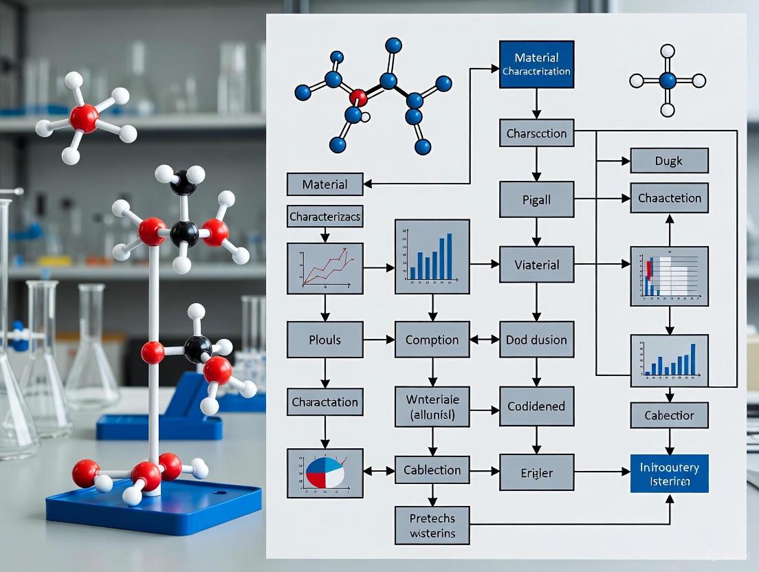
The production of CRMs is governed by international standards, primarily ISO 17034:2016, which outlines the general requirements for the competence of reference material producers [4]. A metrologically valid procedure for certification involves several critical steps to ensure the material is fit for purpose. The diagram below illustrates the established workflow for CRM development and certification, a process that can also be applied to the characterization of RTMs.
Metrological traceability, a requirement for CRMs, is the property of a measurement result whereby it can be related to a reference through a documented, unbroken chain of calibrations, each contributing to the measurement uncertainty [2]. This chain ultimately links the measurement to the International System of Units (SI), ensuring global consistency.
Comparative Analysis: CRMs vs. RMs vs. RTMs
Objective Comparison of Performance and Use Cases
The choice between a CRM, RM, or RTM is dictated by the specific needs of the measurement process, balancing the required level of metrological rigor with practical considerations such as cost and availability. The table below provides a structured comparison of their defining attributes and typical applications.
Table 1: Comparative Overview of CRMs, RMs, and RTMs
| Feature | Certified Reference Material (CRM) | Reference Material (RM) | Reference Test Material (RTM) |
|---|---|---|---|
| Certification & Traceability | Full metrological traceability to SI units; ISO 17034 certified [4] [5] | ISO-compliant, but no mandatory uncertainty or traceability [4] [5] | Characterized, but typically lacks formal certification and traceability [1] [2] |
| Uncertainty Statement | Required; provided for certified values [4] [3] | Not required; may not be provided [4] | May be provided, but not a requirement |
| Primary Documentation | Reference Material Certificate [4] | Product Information Sheet [4] | Data sheet or report from interlaboratory study |
| Ideal Application | Regulatory compliance, method validation, highest precision quantification [4] [5] | Routine quality control, system suitability checks, cost-effective alternative [4] [5] | Method development, interlaboratory comparisons, proficiency testing [1] [2] |
| Cost & Resource Intensity | Higher cost due to rigorous certification [5] | More cost-effective [5] | Varies, often lower cost than CRMs |
Supporting Experimental Data and Validation Context
The critical role of these materials is demonstrated in practice through structured experimental protocols. For instance, the use of a nanoscale CRM for validating a Particle Size Distribution (PSD) measurement by Dynamic Light Scattering (DLS) provides a clear example.
Experimental Protocol 1: Validating DLS Performance with a CRM
- Objective: To validate the accuracy and performance of a DLS instrument for measuring particle size distribution.
- Materials: Nanoscale gold CRM (e.g., NIST RM 8011) with a certified particle size, suitable dispersant.
- Procedure:
- Dispersant Blank: Measure the viscosity and refractive index of the pure dispersant at the controlled measurement temperature.
- CRM Reconstitution: Prepare the CRM according to the certificate's instructions to ensure a monodisperse, stable suspension.
- Instrument Calibration: Follow manufacturer's guidelines for basic optical alignment if required.
- Measurement: Perform a minimum of 3-10 measurement runs of the CRM suspension, ensuring the signal quality meets acceptable thresholds.
- Data Analysis: Record the Z-average hydrodynamic diameter and the polydispersity index (PDI) for each run.
- Validation Criteria: The mean measured Z-average diameter must fall within the expanded uncertainty range of the CRM's certified value. A low PDI confirms the monodispersity of the CRM and proper instrument function.
The data from such an experiment, when summarized, provides objective evidence of measurement validity.
Table 2: Example Data from DLS Validation Using a Gold Nanoparticle CRM
| Measurement Run | Z-Average (d.nm) | Polydispersity Index (PDI) |
|---|---|---|
| CRM Certificate Value | 60.5 ± 2.1 nm | - |
| 1 | 60.9 | 0.05 |
| 2 | 61.5 | 0.04 |
| 3 | 59.8 | 0.06 |
| Mean Experimental Value | 60.7 nm | 0.05 |
| Conclusion | Validation Successful: 60.7 nm lies within the certified uncertainty interval. |
In contrast, RTMs are frequently deployed in Interlaboratory Comparisons (ILCs) to assess the reproducibility of a method across multiple laboratories before it is standardized. An example protocol is outlined below.
Experimental Protocol 2: Assessing Method Reprodubility with an RTM
- Objective: To evaluate the reproducibility of a new analytical method for determining the zeta potential of lipid nanoparticles across multiple laboratories.
- Materials: A single, large batch of well-homogenized lipid nanoparticle RTM, shipped to all participating labs.
- Procedure:
- Protocol Distribution: All participating laboratories receive the same, detailed measurement protocol.
- Sample Distribution: Each lab receives an aliquot from the same batch of the RTM.
- Blinded Measurement: Labs perform zeta potential measurements according to the standard protocol without knowing the expected value.
- Data Submission: All results are submitted to a coordinating body for statistical analysis.
- Outcome Analysis: The collected data is analyzed to determine the between-laboratory reproducibility (standard deviation) and to identify any significant outliers, providing a measure of the method's robustness in real-world conditions.
The Scientist's Toolkit: Essential Research Reagent Solutions
A well-equipped laboratory engaged in materials characterization requires access to a suite of reference materials. The following table details key solutions and their specific functions in the experimental workflow.
Table 3: Essential Research Reagent Solutions for Materials Characterization
| Reagent / Material | Function in Research |
|---|---|
| Inorganic Ion CRM (e.g., for ICP-MS) | Calibration and quantification of elemental concentrations in samples; verifying method accuracy and traceability [5]. |
| Nanoparticle CRM (e.g., Au, SiO₂) | Validating the performance of particle sizing instruments (DLS, NTA), and microscopy for size and shape analysis [1]. |
| Matrix-Matched CRM | Account for matrix effects during analysis; provides a quality control material that closely resembles the sample being tested [5]. |
| Protein or Antibody RM | System suitability testing in chromatographic (e.g., SEC-HPLC) or spectroscopic analyses to monitor column performance and instrument stability. |
| Liposome or Lipid Nanoparticle RTM | Method development and interlaboratory comparison for critical quality attributes (size, zeta potential, encapsulation efficiency) in nanomedicine [1] [2]. |
| Veil-Toughened Composite Preform (e.g., for RTM) | Serves as a consistent reinforcement material for developing and optimizing composite manufacturing processes like Resin Transfer Molding [6] [7]. |
Current Gaps and Future Directions
Despite the critical importance of CRMs and RTMs, significant gaps remain, particularly for novel materials. The current landscape is dominated by spherical nanoparticles with relatively simple compositions and monodisperse size distributions [1] [2]. There is a pressing need for materials that more closely resemble real-world, application-relevant samples.
Key future needs identified in the literature include:
- Complex Morphologies: A lack of CRMs with non-spherical shapes (e.g., rods, cubes, fibers) and high polydispersity [2].
- Advanced Property Certification: Few materials are available with certified values for properties beyond size, such as surface chemistry, surface charge (zeta potential), or particle number concentration [1] [2].
- Complex Matrices: A critical shortage of RMs and CRMs embedded in complex, application-relevant matrices (e.g., biological fluids, environmental samples, consumer products) [1].
- Nanomedicine Standards: The development of lipid-based and other organic nanoparticle RMs is crucial to streamline the regulatory approval process for nanomedicines [1] [2].
Addressing these gaps will require a concerted effort from national metrology institutes, academic researchers, and industry to produce new, fit-for-purpose reference materials that empower the next generation of materials characterization techniques.
Establishing Metrological Traceability to the International System of Units (SI)
In the field of materials characterization, the validity and reliability of experimental data are paramount. Establishing metrological traceability to the International System of Units (SI) ensures that measurements are accurate, comparable, and recognized globally, forming a critical foundation for scientific research and regulatory compliance [8]. This is especially crucial in sectors like drug development, where measurement inconsistencies can directly impact product safety and efficacy. Traceability provides an unbroken chain of comparisons to stated references, typically national or international standards, and is a core requirement of international standards such as ISO/IEC 17025 [8] [9].
This guide objectively compares different frameworks for achieving demonstrable SI traceability, focusing on their application in validating materials characterization techniques. We present supporting experimental data and detailed protocols to help researchers and scientists implement robust measurement systems.
Comparative Frameworks for Achieving Metrological Traceability
Two primary pathways exist for laboratories to demonstrate metrological traceability: accreditation to the international standard ISO/IEC 17025 and participation in specific laboratory recognition programs, such as the one administered by the National Institute of Standards and Technology (NIST) Office of Weights and Measures (OWM) [8] [9].
The following table compares the scope, applicability, and key attributes of the ISO/IEC 17025 standard and the NIST OWM Laboratory Recognition Program, which are central to establishing trust in measurements.
Table 1: Comparison of Metrological Traceability Frameworks
| Feature | ISO/IEC 17025 Accreditation [8] | NIST OWM Laboratory Recognition [9] |
|---|---|---|
| Scope & Applicability | International standard; applicable to all testing and calibration laboratories across all disciplines. | Primarily designed for U.S. state legal metrology laboratories. |
| Primary Focus | Demonstrated technical competence and quality management system of the entire laboratory. | Ensuring SI traceability for state weights and measures programs and addressing specific metrology service issues. |
| Technical Requirements | Validation of methods, estimation of measurement uncertainty, and participation in proficiency testing. | Metrological traceability of standards, documented measurement uncertainties, and use of measurement assurance. |
| Quality System | Requires a full management system, including internal audits and management reviews. | Requires a submitted quality management system and evidence of internal audits and technical reviews. |
| Global Acceptance | Results are accepted internationally under ILAC Mutual Recognition Arrangements (MRA). | Meets state-level legal requirements for traceability in the U.S.; recognition is specific to the U.S. context. |
| Key Impact | Facilitates global trade and acceptance of laboratory results without retesting [8]. | Ensures accurate and uniform measurements for legal metrology and consumer protection within the U.S. |
A significant distinction is that while the general and technical criteria between the two frameworks are nearly identical, the NIST OWM program conducts an annual, targeted analysis of specific metrology services (e.g., mass, volume) and incorporates national findings back into training curricula [9]. This proactive, sector-specific analysis is a distinctive feature of the program.
Experimental Validation of Characterization Techniques
Experimental validation serves as the critical "reality check" for computational models and proposed methodologies [10]. In materials characterization, this often involves using a combination of techniques to cross-verify material properties, from chemical composition to physical behavior.
Case Study: Validating a New Alloy Composition
The table below summarizes quantitative data from a hypothetical study validating the properties of a newly developed titanium-aluminum alloy. The data demonstrates how multiple characterization techniques are used to provide a comprehensive material profile and ensure the results are traceable to SI units.
Table 2: Experimental Data for Validating a New Titanium-Aluminum Alloy
| Characteristic | Target Specification | Experimental Result (Mean ± Uncertainty) | Technique Used | SI-Traceable Reference |
|---|---|---|---|---|
| Aluminum Content | 5.8 - 6.2 atomic % | 6.05 ± 0.15 atomic % | Inductively Coupled Plasma Mass Spectrometry (ICP-MS) | NIST SRM 1250a (Ti Alloy) |
| Yield Strength | ≥ 880 MPa | 895 ± 15 MPa | Uniaxial Tensile Testing | NIST-calibrated load cell & extensometer |
| Young's Modulus | 114 - 120 GPa | 117.5 ± 1.2 GPa | Impulse Excitation Technique | NIST-calibrated frequency reference |
| Grain Size | 10 - 25 µm | 18 ± 3 µm | Scanning Electron Microscopy (SEM) | NIST-traceable magnification standard |
Detailed Experimental Protocol: Alloy Composition and Mechanical Properties
This protocol outlines the key steps for characterizing the alloy's composition and mechanical properties, highlighting points critical for ensuring metrological traceability.
Part A: Chemical Composition via ICP-MS
- Sample Digestion: Precisely weigh 0.1 g of the alloy sample using a calibrated analytical balance. Digest the sample completely in a clean lab environment using high-purity nitric acid (HNO₃) and hydrofluoric acid (HF) in a Teflon vessel.
- Calibration: Prepare a series of calibration standards using a NIST-traceable multi-element standard solution. Include a blank and a control sample (e.g., NIST SRM 1250a) to validate the calibration curve.
- Measurement: Introduce the digested and diluted sample into the ICP-MS. Monitor specific isotopes for Ti and Al.
- Data Analysis: Calculate the atomic percentage of aluminum in the sample based on the calibration curve. Report the result with an estimated measurement uncertainty, incorporating contributions from sample weighing, dilution, and instrument response [11].
Part B: Mechanical Properties via Tensile Testing
- Sample Preparation: Machine tensile test coupons according to ASTM E8/E8M standard specifications. Measure the cross-sectional dimensions of the gauge section using a calibrated micrometer.
- Apparatus Calibration: Verify the calibration of the tensile testing machine's load cell and the extensometer using NIST-traceable reference standards. Confirm the calibration status is current.
- Testing: Mount the coupon in the testing machine and apply a uniaxial load at a specified strain rate until fracture. Simultaneously record load (in Newtons) and elongation (in millimeters) data.
- Data Processing: Convert load and elongation data to engineering stress and strain. Calculate the yield strength (0.2% offset) and Young's modulus from the resulting stress-strain curve. The uncertainty budget must include factors from dimensional measurements, load cell calibration, and data acquisition resolution [12].
Essential Research Reagent Solutions for Materials Characterization
The following table details key reagents, standards, and materials essential for conducting traceable materials characterization, particularly in a pharmaceutical or materials development context.
Table 3: Essential Research Reagent Solutions for Traceable Characterization
| Item | Function / Purpose | Critical for Traceability |
|---|---|---|
| Certified Reference Materials (CRMs) | Provide a known, certified value for a specific property (e.g., elemental concentration, melting point). | Used to calibrate instrumentation and validate analytical methods, creating a direct link to SI units. |
| High-Purity Calibration Standards | Used to prepare calibration curves for spectroscopic techniques (e.g., ICP-MS, Chromatography). | Must be sourced with a certificate of analysis stating traceability to a national metrology institute. |
| NIST-Traceable Standard Reference Materials (SRMs) | A specific type of CRM issued by NIST for verifying the accuracy of measurements. | Serve as the primary anchor for establishing measurement traceability to the SI in the United States [9]. |
| Stable Isotope-Labeled Compounds | Act as internal standards in mass spectrometry to correct for matrix effects and instrument drift. | Improve measurement accuracy and precision, reducing a key component of measurement uncertainty. |
| Standardized Testing Consumables | Includes items like pre-defined fracture toughness coupons or standardized cell culture plates. | Ensure consistency and comparability of physical and biological tests across different laboratories and studies. |
Workflow for Establishing Measurement Traceability
The diagram below outlines the logical workflow for establishing and maintaining metrological traceability for a materials characterization technique, from selecting a method to reporting final results.
Diagram 1: Traceability Establishment Workflow
Interplay of Metrological Concepts in Materials Research
This conceptual diagram illustrates how fundamental metrological concepts interact within the context of materials characterization research to produce reliable and valid data.
Diagram 2: Metrology Concepts in Materials Research
The Critical Role of Homogeneity and Stability in Reference Materials
In the realm of analytical science and materials characterization, reference materials (RMs) serve as essential benchmarks for ensuring measurement accuracy, method validation, and quality control. According to international standards, a reference material is defined as a "sufficiently homogeneous and stable material with respect to one or more specified properties, which has been established to be fit for its intended use in a measurement process" [13]. Similarly, certified reference materials (CRMs) represent the highest standard, characterized by a metrologically valid procedure for specified properties, accompanied by a certificate providing the value, its associated uncertainty, and a statement of metrological traceability [14]. The fundamental role of these materials across diverse fields—from pharmaceutical development to environmental monitoring—hinges on two critical characteristics: homogeneity and stability.
Homogeneity refers to the uniformity of a specified property value throughout a defined portion of a reference material [13]. When materials lack homogeneity, variations between units or within a single unit can introduce significant bias and uncertainty into analytical measurements, compromising the validity of results. Stability, conversely, is the characteristic of a reference material to maintain a specified property value within specified limits for a specified period of time [13]. Without demonstrated stability, the integrity and certified values of a reference material become questionable over time, rendering it unfit for its intended purpose. Together, these properties form the foundation of measurement reliability in research and quality control laboratories worldwide, ensuring that analytical results are comparable across different instruments, laboratories, and time periods [15] [14].
Traditional Methodologies for Assessment
Homogeneity Assessment Approaches
Traditional methods for assessing homogeneity have predominantly relied on statistical techniques capable of detecting variations within and between units of a reference material batch. The Analysis of Variance (ANOVA) has been a cornerstone method, enabling researchers to partition total variability into components attributable to between-unit and within-unit differences [16]. This approach requires a nested experimental design where multiple replicate measurements are taken from multiple units selected randomly from the entire batch.
For sensory analysis of reference materials, such as those used for virgin olive oil, specialized statistical tests are employed. Ranking tests, such as the Page test and 'run' tests, determine whether trained tasters can detect a significant ordering in samples that should theoretically be identical [13]. Similarly, discrimination testing—including 'A-not A' tests, 'triangular' tests, or 'duo-trio' tests—evaluates whether participants can perceive differences between units that might indicate insufficient homogeneity [13]. The fundamental principle underlying these traditional methods is hypothesis testing, where the goal is to demonstrate the absence of statistically significant differences between units at a specified confidence level.
The experimental protocol for traditional homogeneity assessment typically involves:
- Sample Selection: Randomly selecting units from the entire batch population, with a minimum number defined by the formula: ( Nh = \max(10, \sqrt[3]{N{prod}}) ), where ( N_{prod} ) is the total number of units in the batch [13].
- Measurement Design: Implementing a nested design with repeated measurements from each selected unit.
- Statistical Analysis: Applying ANOVA or related statistical tests to quantify between-unit and within-unit variance components.
- Acceptance Criteria: Establishing that between-unit variability does not exceed a predefined fraction of the total measurement uncertainty.
Stability Assessment Approaches
Stability assessment of reference materials focuses on evaluating whether property values remain consistent over time under specified storage conditions. The International Conference on Harmonisation (ICH) has established standardized stability testing protocols that classify the world into four climate zones with specific temperature and humidity conditions for testing [17]. These zones range from temperate (21°C/45%RH) to very hot and humid (30°C/75%RH) environments, ensuring that materials are fit for global use.
Stability studies are typically categorized into three distinct types:
- Influencing Factor Tests: Investigate sensitivity to light, humidity, heat, acid, alkali, and oxidation to understand potential degradation pathways [17].
- Accelerated Tests: Expose materials to elevated stress conditions (e.g., higher temperature and humidity) to rapidly predict long-term stability and shelf life [17].
- Long-Term Tests: Monitor materials under proposed storage conditions to establish expiration dates or retest periods [17].
The experimental protocol for stability assessment includes:
- Sample Preparation: Ensuring test samples are representative of production batches in composition, packaging, and quality [17].
- Storage Conditions: Placing samples in controlled environmental chambers that maintain specific temperature and humidity conditions.
- Time-Point Monitoring: Testing critical quality attributes at predetermined intervals (e.g., 0, 3, 6, 9, 12, 18, 24, 36 months).
- Trend Analysis: Applying statistical methods to detect significant trends in property values over time.
For materials intended for specialized applications, such as implantable medical devices, accelerated reactive aging tests may be employed. These tests use aggressive environments like hydrogen peroxide solutions to simulate long-term stability challenges in a compressed timeframe [18].
Emerging Methods and Innovations
Limitations of Traditional Approaches
While traditional methods like ANOVA have served as the backbone of homogeneity and stability assessment for decades, they present significant limitations when applied to complex modern materials. These limitations become particularly evident with high-dimensional data (such as metagenomic profiles), non-normal distributions, or datasets with temporal components [16]. The reliance on hypothesis testing in traditional approaches often leads to binary "yes/no" determinations about homogeneity or stability, providing little information about the practical significance of observed differences [16]. Furthermore, these methods typically require strict assumptions about data distribution and variance structure that may not hold for complex material systems.
In sensory analysis, traditional methods face the challenge of identifying appropriate "non-homogeneous" reference samples for discrimination testing. When chemical compositions are artificially altered by adding odorant substances to create heterogeneous samples, trained tasters may recognize the differences as originating from exogenous compounds rather than representing genuine heterogeneity in the material [13]. This fundamental limitation complicates the validation of homogeneity for sensory reference materials.
Innovative Assessment Approaches
Coefficient of Disagreement
A novel approach termed the coefficient of disagreement has been proposed to address limitations of traditional methods. Instead of testing for statistically significant differences, this method focuses on a more practical question: "If you chose two samples at random from the population, how different could the values be for properties of interest?" [16]. This approach characterizes the expected variability between random sample pairs, providing researchers with directly interpretable information about the level of disagreement they might encounter when using different units of the same reference material.
The coefficient of disagreement offers several advantages:
- Practical Interpretation: Provides tangible information about expected measurement variability rather than statistical significance.
- Flexibility: Can be applied to various data types, including high-dimensional and non-normal distributions.
- Risk Assessment: Enables users to evaluate whether the observed variability is acceptable for their specific application.
High-Throughput Mechanical Characterization
In metallurgical materials, innovative approaches using isostatic pressing have been developed for high-throughput characterization of mechanical homogeneity [19]. This technique applies uniform pressure to material surfaces and analyzes the resulting strain patterns to identify microregions with poor mechanical properties. The method involves:
- Surface Preparation: Grinding and polishing samples until no obvious scratches are detectable.
- Baseline Characterization: Mapping elemental content, microstructure, defects, and 3D surface morphology.
- Strain Application: Subjecting samples to cold isostatic pressing (CIP) with controlled pressure and duration.
- Strain Analysis: Comparing surface profiles before and after pressing to identify microregions with abnormal strain behavior.
This approach enables statistical characterization of micromechanical properties across full surfaces, identifying weak interfaces, non-metallic inclusions, pores, and other defects that might compromise material performance [19].
Comparative Analysis of Methods
Table 1: Comparison of Traditional and Emerging Assessment Methods
| Method Category | Specific Technique | Application Scope | Data Requirements | Key Advantages | Principal Limitations |
|---|---|---|---|---|---|
| Traditional Homogeneity | Analysis of Variance (ANOVA) | Univariate properties, normal data | Balanced nested design | Well-established statistical framework | Limited with complex, high-dimensional data |
| Traditional Homogeneity | Sensory Ranking Tests | Foodstuffs, sensory panels | Trained panelists | Direct assessment of perceivable differences | Subjective, requires extensive training |
| Traditional Stability | Accelerated Testing | Shelf-life prediction | Multiple time points | Rapid results | Extrapolation uncertainties |
| Traditional Stability | Long-term Testing | Real-time stability | Extended monitoring period | Direct evidence under actual conditions | Time-consuming |
| Emerging Methods | Coefficient of Disagreement | Complex, high-dimensional data | Paired sample comparisons | Intuitive interpretation | Less familiar to traditionalists |
| Emerging Methods | Isostatic Pressing | Metallurgical materials | Surface profile data | High-throughput capability | Specialized equipment requirements |
Table 2: Stability Testing Conditions Based on Climate Zones
| Climate Zone | Description | Long-term Testing Conditions | Accelerated Testing Conditions | Primary Geographical Regions |
|---|---|---|---|---|
| I | Temperate | 21°C/45%RH | Not specified | Various temperate regions |
| II | Subtropical | 25°C/60%RH | 40°C/75%RH | ICH regions, subtropical areas |
| III | Dry heat | 30°C/35%RH | Not specified | Dry climate regions |
| IVA | Hot and humid | 30°C/65%RH | Not specified | Hot, humid tropical regions |
| IVB | Very hot and humid | 30°C/75%RH | Not specified | Very hot, humid tropical regions |
Experimental Protocols in Practice
Detailed Protocol: Homogeneity Assessment of Liquid Foodstuffs
The homogeneity assessment of virgin olive oil reference materials for sensory analysis follows a meticulously designed protocol:
Sample Preparation: Obtain representative samples from the candidate reference material batch, ensuring they are stored in identical containers under controlled conditions [13].
Panel Selection and Training: Engage 8-12 trained tasters who have been harmonized in sensory detection and quantification of relevant attributes. The panel must demonstrate high precision in previous validation studies [13].
Experimental Design:
- For ranking tests: Present samples in randomized order to each taster, who must rank them based on intensity of specific attributes.
- For discrimination tests: Present paired samples (target/reference and test samples) in balanced designs to avoid sequence bias.
Statistical Analysis:
- Apply Page test for trend detection in rankings: ( L = \sum{j=1}^{k} (Rj \times j) ), where ( R_j ) is the sum of ranks for group j.
- Use runs test to identify non-random patterns: ( Z = \frac{R - \overline{R}}{s_R} ), where R is the number of runs.
- For discrimination tests, apply binomial tests to determine if misclassification rates exceed chance levels.
Interpretation: Consider samples homogeneous when ranking appears random or when misclassification rates lack statistical significance at α=0.05.
Detailed Protocol: Accelerated Reactive Aging Test for Implantable Devices
The assessment of packaging material stability for neural implants using accelerated reactive aging tests involves:
Sample Preparation: Coat tungsten wires (50µm diameter) with various packaging materials (Parylene C, SiO2, Si3N4) using chemical vapor deposition or plasma-enhanced chemical vapor deposition [18].
Experimental Groups: Prepare both closed-tip and open-tip configurations with varying coating thicknesses and material combinations.
Accelerated Aging: Immerse samples in three solutions at approximately 67°C:
- pH 7.4 phosphate-buffered saline (PBS)
- PBS + 30 mM H₂O₂
- PBS + 150 mM H₂O₂
Monitoring: Measure electrochemical impedance spectroscopy (EIS) regularly, noting when impedance at 1 kHz changes by >50% of initial value.
Failure Analysis: Use scanning electron microscopy to examine physical damage, pinholes, cracks, and interface delamination at failure points.
Data Modeling: Apply Weibull distribution analysis to calculate mean-time-to-failure (MTTF) and cumulative failure probability over time [18].
Visualization of Methodologies
Homogeneity Assessment Workflow
Reference Material Validation Pathway
The Scientist's Toolkit: Essential Research Reagent Solutions
Table 3: Essential Reagents and Materials for Homogeneity and Stability Studies
| Reagent/Material | Function | Application Examples | Key Considerations |
|---|---|---|---|
| Saturated Salt Solutions | Maintain constant humidity in closed containers | Influencing factor tests, stability studies | NaCl sat. solution: 75%RH (15.5-60°C); KNO3 sat. solution: 92.5%RH (25°C) [17] |
| Certified Reference Materials | Quality control for analytical method validation | Method development, accuracy verification | Matrix-matched CRMs preferred; assess extraction efficiency, interfering compounds [14] |
| Hydrogen Peroxide Solutions | Accelerated reactive aging medium | Implantable device packaging stability | PBS + 30mM H₂O₂ and PBS + 150mM H₂O₂ simulate inflammatory response [18] |
| Standardized Light Sources | Photostability testing | Influencing factor tests for light sensitivity | D65/ID65 emission standard; daylight fluorescent, xenon, or metal halide lamps [17] |
| Isostatic Pressing Equipment | High-throughput mechanical screening | Metallurgical material homogeneity | Apply uniform pressure (190MPa) to identify weak microregions [19] |
| Environmental Chambers | Controlled stability conditions | Long-term and accelerated testing | Precise temperature/humidity control for ICH climate zones [17] |
The critical role of homogeneity and stability in reference materials cannot be overstated, as these properties fundamentally determine the reliability and traceability of analytical measurements across scientific disciplines. While traditional assessment methods like ANOVA and accelerated stability testing have established a strong foundation for reference material certification, emerging approaches such as the coefficient of disagreement and high-throughput mechanical characterization offer enhanced capabilities for complex modern materials. The continued evolution of assessment methodologies will further strengthen the metrological infrastructure, supporting advances in materials characterization, pharmaceutical development, and analytical science. As reference materials grow increasingly sophisticated to meet the demands of modern research, so too must the methods for verifying their homogeneity and stability, ensuring they remain fit for purpose in validating materials characterization techniques.
Navigating International Standards and Regulatory Guidelines
In the fields of materials science and pharmaceutical development, the validation of materials characterization techniques is fundamental to establishing reliable structure-activity relationships and ensuring product quality, safety, and efficacy. Advanced characterization techniques, spanning from the micro-nano to the atomic scale, serve as powerful foundation tools for investigating and understanding material properties and functions [20]. As structural complexity increases across advanced alloys, composite materials, and novel drug delivery systems, researchers face mounting challenges in accurately characterizing material properties across different scales [21]. The current landscape is further complicated by the proliferation of new materials and manufacturing processes, which demand efficient, reproducible, and standardized characterization protocols to bridge the gap between innovative research and regulatory compliance.
This guide provides a comprehensive comparison of characterization techniques and methodologies, with a specific focus on their validation under international standards and regulatory frameworks. We present structured experimental data, detailed protocols, and analytical workflows to assist researchers in selecting appropriate techniques, optimizing measurement parameters, and demonstrating methodological rigor for both scientific publication and regulatory submissions.
Comparative Analysis of Major Characterization Techniques
A diverse array of characterization techniques is employed to decipher material properties, each with specific strengths, limitations, and applications in regulated environments. The following comparison covers major technique categories relevant to modern materials and biopharmaceutical research.
Table 1: Comparison of Primary Materials Characterization Techniques
| Technique | Primary Information | Spatial Resolution | Standards (Typical) | Key Regulatory Applications |
|---|---|---|---|---|
| XRD (X-ray Diffraction) | Crystal structure, phase identification, residual stress | Macroscopic to ~1 µm (lab source) | ASTM E915, ISO 22278 | Pharmaceutical polymorph identification, alloy phase verification [21] [22] |
| SEM/TEM (Scanning/Transmission Electron Microscopy) | Morphology, microstructure, elemental composition (with EDS) | SEM: ~1 nm; TEM: <0.1 nm | ISO 16700, ASTM E986 | LNP morphology, particle size distribution, defect analysis [20] [23] |
| XPS (X-ray Photoelectron Spectroscopy) | Surface chemical composition, oxidation states | ~10 µm (lab source) | ISO 15470, ASTM E902 | Surface chemistry of biomaterials, coating analysis [20] [21] |
| AFM (Atomic Force Microscopy) | Surface topography, nanomechanical properties | Lateral: ~1 nm; Vertical: ~0.1 nm | ISO 27911 | Surface roughness of medical devices, nanotexture analysis [23] |
| NMR (Nuclear Magnetic Resonance) | Molecular structure, dynamics, quantitative composition | Atomic scale (no spatial resolution) | USP <761>, ICH Q3D | Drug molecule structure confirmation, impurity profiling [20] |
| EDS/EELS (Energy Dispersive X-ray Spectroscopy/Electron Energy-Loss Spectroscopy) | Elemental composition, chemical bonding | EDS: ~1 µm; EELS: sub-nm | ISO 22309 | Elemental analysis in composites, contamination identification [20] [23] |
Advanced and Emerging Technique Capabilities
Table 2: Advanced and In-Situ Characterization Techniques
| Technique | Unique Capabilities | Data Complexity | Regulatory Readiness | Specialized Applications |
|---|---|---|---|---|
| FIB-SEM Tomography | 3D reconstruction of microstructures with nanometric resolution [21] | High (requires specialized data processing) | Emerging (reference methodologies needed) | Pore network analysis in batteries, fuel cells [21] |
| Atom Probe Tomography (APT) | 3D atomic-scale elemental mapping | Very High (complex data interpretation) | Research Phase | Nanoscale precipitation in alloys, interfacial analysis [23] |
| Cryo-EM (Cryo-Electron Microscopy) | High-resolution imaging of biological specimens in vitreous ice | High (requires specialized sample prep) | Mature for biologics | LNP structure, virus-like particles, protein complexes [23] |
| In Situ/Operando XRD | Real-time monitoring of structural changes under external stimuli [20] | Medium-High (complex experiment design) | Growing adoption | Phase transformation kinetics (e.g., TRIP steels), battery material degradation [20] [22] |
Experimental Protocols for Technique Validation
Validated experimental protocols are essential for generating reliable, reproducible data that meets regulatory scrutiny. This section details methodologies for key characterization scenarios, emphasizing measurement optimization and standardization.
Protocol 1: Retained Austenite Analysis in Advanced High-Strength Steels
Objective: To quantitatively determine the phase fraction of retained austenite in a Quench and Partitioning (QP) steel using energy-dispersive X-ray diffraction (XRD) with minimized measurement time while maintaining data quality [22].
Materials and Reagents:
- Material: Low-alloy 42CrSi QP steel sample (dog-bone-shaped tensile specimen with gauge section dimensions of 18 × 3 × 1 mm³) [22]
- Equipment: Energy-dispersive X-ray diffractometer, Kammrath & Weiss stress rig for in situ loading [22]
- Software: Data acquisition system with capability for real-time data evaluation and custom scripting for region-of-interest (ROI) analysis [22]
Methodology:
- Sample Preparation: Austinitize sample at 950°C, quench to 170°C in liquid salt, followed by partitioning at 400°C for 10 minutes [22]. Prepare final specimen using electrical discharge machining (EDM).
- Initial Measurement Parameters: Set up diffraction experiment with initial exposure time sufficient to detect major ferrite and austenite peaks (e.g., {110}, {200} for ferrite; {111}, {200} for austenite).
- Data Collection Strategies:
- Traditional Sequential Acquisition: Collect data across the entire energy range with fixed, sufficiently long counting times (state-of-the-art, used as benchmark) [22].
- Regions-of-Interest (ROI) Strategy: Focus counting time on specific energy ranges corresponding to the most relevant diffraction peaks for the analysis (e.g., peaks for quantitation of austenite fraction) [22].
- Minimum Volume Strategy: Dynamically select the next energy interval to measure based on the minimal information gained from previously acquired data points to maximize information per unit time [22].
- Data Analysis: Integrate peak intensities for relevant diffraction planes. Calculate retained austenite volume fraction using direct comparison method, accounting for crystallographic structure factors [22].
- Termination Criteria: Implement real-time data quality assessment to determine when sufficient data has been collected for a predetermined accuracy threshold (e.g., <2% relative error in phase fraction), avoiding redundant measurements [22].
Validation Parameters: Precision of phase fraction measurement, signal-to-background ratio of diffraction peaks, total experiment time, and correlation with reference methods (e.g., EBSD) [22].
Protocol 2: Comprehensive Characterization of Lipid Nanoparticles (LNPs)
Objective: To perform thorough physicochemical characterization of mRNA-loaded Lipid Nanoparticles (LNPs) using a suite of orthogonal techniques, establishing key critical quality attributes (CQAs) for regulatory submission [24].
Materials and Reagents:
- Material: LNP formulation composed of ionizable lipid, phospholipid, cholesterol, and PEG-lipid, loaded with mRNA payload [24]
- Standards: USP <729> for globule size distribution, ICH Q2(R1) for analytical method validation
- Equipment: Nanoparticle Tracking Analysis (NTA) or Dynamic Light Scattering (DLS) for size, TEM for morphology, HPLC for encapsulation efficiency [24]
Methodology:
- Particle Size and Distribution:
- Use DLS for hydrodynamic diameter and polydispersity index (PDI)
- Employ NTA for concentration and particle size distribution in complex biological fluids
- Perform measurements in triplicate at 25°C following standard operating procedure based on USP <729>
- Encapsulation Efficiency:
- Implement ribonucleic acid (RNA) binding assay (e.g., using Ribogreen dye) to distinguish encapsulated vs. free RNA
- Validate assay specificity, linearity, and precision per ICH Q2(R1) guidelines
- Calculate encapsulation efficiency as: (Total RNA - Free RNA)/Total RNA × 100%
- Morphological Analysis:
- Prepare samples for TEM using negative staining with uranyl acetate
- Acquire images at multiple magnifications to assess particle morphology, uniformity, and potential aggregates
- Use image analysis software to quantify morphological parameters from at least 100 particles
- Surface Functionalization Analysis:
- Employ XPS to verify surface composition and successful functionalization (e.g., with targeting ligands)
- Use ζ-potential measurements to assess surface charge changes after modification
- Stability Assessment:
- Monitor size, PDI, and encapsulation efficiency over time under accelerated storage conditions (e.g., 4°C, 25°C/60% RH)
- Establish specifications for shelf-life determination
Validation Parameters: Method precision (RSD < 10% for size measurements), accuracy (recovery 90-110% for encapsulation efficiency), linearity (R² > 0.98 for analytical curves), and robustness (deliberate variations in method parameters) [24].
Visualization of Characterization Workflows
The following diagrams illustrate standardized workflows for materials characterization, highlighting decision points, technique selection criteria, and data integration strategies essential for regulatory compliance.
Logical Framework for Characterization Technique Selection
Figure 1: Technique Selection Framework - A systematic approach for selecting appropriate characterization techniques based on information requirements, analysis scale, sample limitations, and regulatory context.
Materials Testing 2.0 Integrated Workflow
Figure 2: MT 2.0 Calibration Workflow - NIST's "Materials Testing 2.0" inverse approach for efficient material model calibration using a single complex experiment combined with FEA simulation, replacing multiple traditional tests [25].
The Scientist's Toolkit: Essential Research Reagent Solutions
Table 3: Key Reagents and Materials for Characterization Experiments
| Item/Category | Function/Purpose | Application Examples | Standards Compliance |
|---|---|---|---|
| Ionizable Lipids | Structural component of LNPs for nucleic acid encapsulation and delivery [24] | mRNA vaccine delivery systems, gene therapies | cGMP manufacturing, regulatory filings for novel excipients |
| Gemini Surfactants | Pore-forming templates for mesoporous material synthesis [21] | Mesoporous silica sieves for water remediation, drug delivery | EPA guidelines for environmental applications |
| Hydroxyapatite (Eggshell-derived) | Biomedical scaffold material resembling human bone [21] | Bone tissue engineering, orthopedic implants | ASTM F2027 (characterization of tissue-engineered medical products) |
| Reference Materials | Calibration and method validation | Instrument qualification, measurement traceability | NIST traceable, ISO 17025 accredited sources |
| Stable Isotope Labels | Tracers for quantitative mass spectrometry | Pharmacokinetic studies, metabolic pathway analysis | USP <1065> for isotope-containing compounds |
Current Gaps and Future Needs in Nanoscale Reference Materials
The rational design and safe application of engineered nanomaterials (NMs) across consumer products, medical diagnostics, drug delivery, and environmental technologies demand reliable, validated characterization methods for key physicochemical properties [2] [1]. These properties include particle size, size distribution, shape, surface chemistry, and particle number concentration, which collectively determine nanomaterial functionality, safety, and environmental impact [1]. The validation of characterization methods used for these properties relies critically on the availability of high-quality nanoscale reference materials (RMs), certified reference materials (CRMs), and reference test materials (RTMs) [2] [1]. These materials serve as benchmarks for instrument calibration, method validation, and interlaboratory comparisons, ensuring measurement comparability and result reliability, which are especially crucial in regulated areas like nanomedicine [2] [26]. Despite their importance, significant gaps persist in the availability of such materials, limiting the progress of nanotechnology and the implementation of safe-and-sustainable-by-design (SSbD) concepts [2] [1] [26]. This guide objectively compares the current landscape of available nanoscale reference materials against identified needs, detailing the limitations and recent progress in this critical field.
The Critical Role and Definitions of Reference Materials
Reference materials are high-quality, comprehensively characterized samples that laboratories use to control and calibrate instruments, develop new measurement methods, and ensure results are reliable and comparable [26]. Within this broad category, specific definitions and quality criteria exist, establishing a metrological hierarchy:
- Certified Reference Material (CRM): The gold standard, defined by ISO as a "material characterized by a metrologically valid procedure, accompanied by a certificate specifying the property value along with a statement of metrological traceability" [2]. Metrological traceability requires an unbroken chain of calibrations linking the measurement to an SI unit, with stated uncertainties for each step.
- Reference Material (RM): A material that is "sufficiently homogeneous and stable with respect to one or more specified properties" and is fit for its intended measurement purpose [2]. While often accompanied by detailed reports, RMs do not require a full uncertainty estimation or metrological traceability.
- Reference Test Material (RTM) or Quality Control (QC) Material: Well-characterized materials, often assessed in interlaboratory comparisons (ILCs), which are stable and homogeneous for specific application-relevant properties. They are vital for method development and standardization, even in the absence of full traceability [2] [1].
The certification process for CRMs is resource-intensive, typically led by national metrology institutes (NMIs), and involves material selection, stability and homogeneity assessment, and characterization using metrologically valid procedures [2].
Current Landscape and Limitations of Available Nanoscale Reference Materials
Despite the increasing use of engineered nanomaterials, adequate characterization data are often lacking, hampering the comparability of measurements and the value of toxicity studies [2]. A review of the current state reveals that available CRMs and RMs are predominantly spherical nanoparticles with relatively monodisperse size distributions and certified values for basic properties like particle size or specific surface area [2]. Table 1 summarizes the primary limitations and gaps in the existing portfolio of nanoscale reference materials.
Table 1: Major Gaps in Currently Available Nanoscale Reference Materials
| Gap Category | Specific Limitation | Impact on Research and Industry |
|---|---|---|
| Shape and Polydispersity | Scarcity of non-spherical shapes (e.g., rods, cubes) and materials with high polydispersity [2] [26]. | Hinders validation of size measurements for complex morphologies and accurate determination of particle number concentration [2]. |
| Certified Properties | Focus on size/surface area; lack of CRMs for surface chemistry, particle number concentration, and zeta potential [2] [1] [26]. | Impedes reliable risk assessment and functionality evaluation, which are heavily influenced by surface properties [1]. |
| Material Complexity | Few materials representing core-shell structures, hybrid materials, or organic nanomaterials like liposomes [2] [1]. | Limits applicability to real-world, commercially available nano-formulations, especially in nanomedicine [2]. |
| Application-Relevant Matrices | Most RMs are in simple suspensions, ill-suited for complex matrices (e.g., biological fluids, environmental samples, consumer products) [2] [1]. | Prevents accurate characterization and monitoring of NMs in their actual end-use environments or for fate and exposure studies [1]. |
These gaps have direct consequences. The lack of reference materials with known surface chemistry, for instance, is a critical barrier for nanomaterial risk assessment and for the development of effective nanomedicines, where surface functionality dictates biological interactions [26] [27]. Furthermore, the disparity in regulatory definitions of nanomaterials between jurisdictions (e.g., EU vs. USA) complicates global approval processes, a situation that could be mitigated by standardized measurement methods traceable to common reference materials [1].
Experimental Protocols for Reference Material Certification and Characterization
The development of a certified reference material is a rigorous process that employs a suite of characterization techniques to assign certified values with metrological traceability. The following workflow and detailed methodologies outline how key experiments are conducted to validate nanomaterial properties.
Table 2: Key Experimental Protocols for Characterizing Nanoscale Reference Materials
| Property | Primary Characterization Method | Experimental Protocol & Key Details |
|---|---|---|
| Particle Size & Morphology | Transmission Electron Microscopy (TEM) / Scanning Electron Microscopy (SEM) [28] | Protocol: Samples are deposited on TEM grids or SEM substrates. Multiple images are taken systematically across the grid. For each particle, dimensions are measured. Data Analysis: Size distribution is generated from measuring hundreds to thousands of particles. Values reported as mean diameter, median, and standard deviation or D50, D10, D90 [28]. |
| Chemical Composition | Energy Dispersive X-Ray Spectroscopy (EDS/EDX) [28] | Protocol: Often coupled with SEM/TEM. An electron beam excites the sample, emitting element-specific X-rays. Data Analysis: Spectral peaks identify elements; peak intensities quantify composition. Provides elemental mapping to show distribution [28]. |
| Surface Chemistry | X-ray Photoelectron Spectroscopy (XPS) [28] | Protocol: A solid surface is irradiated with an X-ray beam, ejecting photoelectrons. The kinetic energy of these electrons is measured. Data Analysis: Binding energy identifies elements and their chemical states (e.g., oxidized vs. metallic). The analysis depth is limited to 1-10 nm, making it ideal for surface characterization [28]. |
| Crystal Structure | X-ray Diffraction (XRD) [12] | Protocol: A collimated X-ray beam is incident on the nanomaterial powder or film. The diffracted intensity is measured as a function of the scattering angle. Data Analysis: The position of diffraction peaks identifies the crystal phase, and peak broadening is used to estimate crystallite size via the Scherrer equation [12]. |
| Surface Charge | Zeta Potential Measurement [1] | Protocol: The nanomaterial dispersion is placed in a cell with electrodes. An electric field is applied, and the velocity of moving particles (electrophoretic mobility) is measured via laser Doppler velocimetry. Data Analysis: The Henry equation is used to convert electrophoretic mobility to zeta potential, indicating colloidal stability [1]. |
| Specific Surface Area | Brunauer-Emmett-Teller (BET) Method [2] | Protocol: The nanomaterial sample is degassed under vacuum to remove contaminants. The amount of nitrogen gas adsorbed onto the surface is measured at various pressures at liquid nitrogen temperature. Data Analysis: The BET model is applied to the adsorption isotherm to calculate the specific surface area [2]. |
Recent Developments and Comparative Analysis of New Reference Materials
Recent projects have begun to address the critical gaps outlined in Table 1. Two significant developments highlight the direction of progress:
- Iron Oxide Nanocubes (BAM, Germany): This CRM addresses the critical gap for non-spherical shapes [26] [27]. Unlike traditionally available spherical nanoparticles, the cubic shape allows for validating methods that are sensitive to particle morphology. These materials are relevant for applications in magnetic resonance imaging (MRI) and demonstrate that shape-specific reference materials are now achievable.
- Lipid-Based Nanoparticles (NRC, Canada): This development tackles the gap for organic nanomaterials and complex compositions relevant to nanomedicine [2] [26] [27]. Lipid nanoparticles are crucial carrier systems for drugs and vaccines (e.g., COVID-19 mRNA vaccines). The availability of an RM for such a complex, organic-based system is a pivotal step towards ensuring the quality, safety, and efficacy of nanomedicines.
Table 3 provides a comparative analysis of these new materials against traditional options and ideal future materials.
Table 3: Comparison of Nanoscale Reference Material Generations
| Material Feature | Traditional RMs (e.g., Spherical Gold/Silica NPs) | Recent Advanced RMs (e.g., BAM Nanocubes, NRC Liposomes) | Ideal Future RMs (Unmet Needs) |
|---|---|---|---|
| Shape | Predominantly spherical [2] | Non-spherical (e.g., cubes) [26] | Mixed shapes, high-aspect-ratio (rods, plates) |
| Surface Chemistry | Limited or no certified data [2] [26] | Partially addressed in new projects (e.g., SMURFnano) [26] | Certified values for functional groups, coating density |
| Composition | Inorganic, single-component | Complex organic & hybrid (lipids, polymers) [2] [26] | Core-shell, multicomponent, hybrid materials |
| Matrix | Simple aqueous suspension | Simple aqueous suspension | Complex matrices (serum, soil, food) [2] [1] |
| Certified Properties | Size, Specific Surface Area [2] | Size, Shape | Particle Number Concentration, Surface Chemistry, Bioreactivity [2] [26] |
The Scientist's Toolkit: Essential Research Reagent Solutions
The characterization of nanoscale reference materials and the development of new nanomaterials rely on a suite of advanced analytical techniques and reagents. The following table details key solutions and their functions in this field.
Table 4: Essential Research Reagent Solutions for Nanomaterial Characterization
| Tool / Reagent Category | Specific Examples | Primary Function in Characterization |
|---|---|---|
| Microscopy | Scanning Electron Microscope (SEM), Transmission Electron Microscope (TEM), Atomic Force Microscope (AFM) [12] [28] [29] | Provides high-resolution imaging of particle size, shape, morphology, and aggregation state. AFM can also measure nanomechanical properties [29]. |
| Elemental & Surface Analysis | Energy Dispersive X-Ray Spectroscopy (EDS), X-ray Photoelectron Spectroscopy (XPS) [28] | EDS determines elemental composition; XPS provides quantitative chemical state information from the top 1-10 nm of a material's surface [28]. |
| Particle Analysis Software | Automated Particle Workflow (APW), Avizo Software [28] | Automates the acquisition and analysis of large datasets from SEM/TEM, providing statistically significant size and composition distributions [28]. |
| Sample Preparation | Focused Ion Beam (FIB) Systems [28] | Enables precise cross-sectioning and preparation of thin samples for TEM analysis, crucial for examining core-shell structures or internal defects. |
| Stable Nanomaterial Dispersions | Buffer solutions with specific ionic strength and pH, surfactants | Maintains colloidal stability of nanomaterial RMs during characterization, preventing aggregation that would skew size measurements. |
The path forward for nanoscale reference materials requires a concerted effort from the international metrology and nanotechnology communities. Key priorities include:
- Multi-Measurand RMs: Developing materials that come with certified values for multiple properties (e.g., size, shape, surface chemistry, and number concentration) to maximize utility and efficiency for end-users [2].
- Materials for Complex Matrices: A critical need exists for RMs that mimic real-world conditions, such as nanomaterials embedded in polymer composites, suspended in biological fluids, or present in environmental samples [2] [1]. This is essential for validating methods used in environmental monitoring, toxicology, and product quality control.
- Enhanced Data Accessibility: Making reliable characterization data readily available in open, standardized databases will accelerate development and ensure the safe use of nanomaterials [26].
- Addressing Legislative Needs: The development of RMs for particle number concentration is urgently needed to support new EU legislative requirements, highlighting the growing link between metrology and regulation [2].
In conclusion, while recent developments like iron oxide nanocubes and lipid-based nanoparticle RMs represent significant progress, the current landscape of nanoscale reference materials is characterized by critical gaps that hinder the reliable characterization, regulation, and commercialization of engineered nanomaterials. Closing these gaps through the targeted development of more complex, application-relevant, and multi-faceted reference materials is essential for unlocking the full potential of nanotechnology across medicine, electronics, and environmental applications, ensuring both functionality and safety.
Advanced Techniques and Sector-Specific Applications in Biomedicine and Materials Science
Applying Primary Difference Methods (PDM) and Classical Primary Methods (CPM) for High-Accuracy Analysis
The integrity of chemical measurement results, particularly in fields like pharmaceutical development and environmental monitoring, depends on rigorous metrological traceability to the International System of Units (SI) [30]. Certified reference materials (CRMs), especially monoelemental calibration solutions, form the critical link between abstract SI definitions and practical analytical measurements [31] [30]. The characterization of these primary standards employs two principal methodological approaches: Classical Primary Methods (CPM) and Primary Difference Methods (PDM) [31] [30]. CPMs, such as titrimetry or coulometry, directly assay the analyte's mass fraction, while PDMs indirectly determine purity by quantifying and subtracting all impurities from an ideal 100% value [31] [30]. Framed within a broader thesis on validating materials characterization techniques, this guide objectively compares the performance of PDM and CPM through experimental data from a bilateral comparison between national metrology institutes (NMIs). The findings demonstrate that despite fundamentally different principles and traceability paths, both methods achieve excellent agreement, underscoring their reliability in producing SI-traceable reference values for high-accuracy analysis [31].
Methodological Principles and Traceability
The core distinction between CPM and PDM lies in their analytical approach to certifying the purity of a high-purity material or the mass fraction in a calibration solution.
Classical Primary Methods (CPM) are direct analytical procedures that quantify the main analyte without requiring a reference standard of the same kind [30]. Gravimetric titration, a prominent CPM, involves directly assaying the element of interest in a solution using a well-characterized titrant. The measurement result is traceable to the SI through the mole and highly accurate mass determinations [31].
Primary Difference Methods (PDM) are indirect procedures that certify a material's purity by quantifying all possible metallic and non-metallic impurities and subtracting their sum from the ideal purity of 1 kg/kg [31] [30]. This "reverse" approach bundles many individual measurements and is universally applicable to all elements [30]. The subsequent use of this certified primary standard in the gravimetric preparation of a calibration solution provides the pathway for SI traceability [31].
The following workflow diagrams illustrate the distinct but complementary traceability chains for these two methods.
Traceability Workflow for Classical Primary Methods (CPM)
Traceability Workflow for Primary Difference Methods (PDM)
Experimental Comparison: Cadmium Calibration Solutions
A bilateral comparison between the NMIs of Türkiye (TÜBİTAK-UME) and Colombia (INM(CO)) provides a robust dataset to evaluate the performance of PDM and CPM [31]. Each institute independently produced a cadmium monoelemental calibration solution with a nominal mass fraction of 1 g/kg and characterized both their own solution and the other's using their preferred primary method.
Table 1: Key experimental parameters and methodologies used in the bilateral comparison [31].
| Parameter | TÜBİTAK-UME (Employing PDM) | INM(CO) (Employing CPM) |
|---|---|---|
| Methodology | Primary Difference Method (PDM) | Classical Primary Method (CPM) |
| Primary Method | Impurity assessment via HR-ICP-MS, ICP-OES, and CGHE | Gravimetric complexometric titration with EDTA |
| CRM Prepared | UME-CRM-2211 | INM-014-1 |
| Cadmium Source | Granulated high-purity Cd metal (Alfa Aesar, Puratronic) | High-purity Cd metal foil (Sigma-Aldrich) |
| Acid Used | Purified nitric acid (~2% final mass fraction) | Purified nitric acid (~2% final mass fraction) |
| Value Assignment | Combination of gravimetry and HP-ICP-OES | Direct assay via titration |
| Key Techniques | HR-ICP-MS, ICP-OES, Carrier Gas Hot Extraction (CGHE) | Gravimetric titration |
Detailed Experimental Protocols
- Impurity Assessment: The purity of a granulated cadmium metal standard was determined using a PDM. This involved the development and validation of methods for 73 elemental impurities.
- Techniques: High-Resolution Inductively Coupled Plasma Mass Spectrometry (HR-ICP-MS), Inductively Coupled Plasma Optical Emission Spectrometry (ICP-OES), and Carrier Gas Hot Extraction (CGHE).
- Quantification: Commercial multi-element standard solutions were used as calibrants. Impurities below the limit of detection (LOD) were assigned a mass fraction value of half the LOD, with a 100% relative uncertainty.
- Gravimetric Preparation: The certified high-purity cadmium metal was dissolved in purified nitric acid and diluted with ultrapure water (resistivity >18 MΩ cm) under full gravimetric control to produce solution UME-CRM-2211.
- Confirmation with HP-ICP-OES: High-Performance ICP-OES was used to confirm the cadmium mass fraction in the gravimetrically prepared solution, providing a second traceable measurement result.
- Titrant Characterization: The ethylenediaminetetraacetic acid (EDTA) salt used as the titrant was first characterized by titrimetry to establish its own purity and ensure traceability.
- Direct Assay by Titration: The cadmium mass fraction in both its own solution (INM-014-1) and the solution received from TÜBİTAK-UME (UME-CRM-2211) was directly determined using gravimetric complexometric titration with the characterized EDTA.
- Solution Preparation: The INM-014-1 solution was prepared by dissolving pre-cleaned high-purity cadmium metal foil in purified nitric acid, followed by dilution with ultrapure water and aliquoting into sealed glass ampoules.
Comparative Performance Data and Results
The culmination of the bilateral comparison demonstrated a high level of technical competency and methodological validation for both approaches.
Results and Uncertainty Comparison
Table 2: Comparison of assigned values, uncertainties, and key outcomes from the bilateral study [31].
| Comparison Metric | TÜBİTAK-UME (PDM) | INM(CO) (CPM) | Assessment |
|---|---|---|---|
| Value for UME-CRM-2211 | Assigned via PDM/gravimetry/HP-ICP-OES | Confirmed by CPM (Titration) | Excellent agreement within stated uncertainties |
| Value for INM-014-1 | Measured by HP-ICP-OES | Assigned by CPM (Titration) | Excellent agreement within stated uncertainties |
| Achievable Uncertainty | Very low (< 0.01% or 10⁻⁴ relative uncertainty) [30] | Low (typical of high-accuracy titration) | PDM can achieve exceptionally low uncertainties |
| Metrological Compatibility | Yes | Yes | Results are metrologically equivalent |
| Key Advantage | Universal applicability; ultra-low uncertainties | Direct measurement principle | Both provide SI traceability |
The measurement results for the cadmium mass fraction in the solutions, as determined by both institutes using their independent methods, exhibited excellent agreement within their stated uncertainties [31]. This outcome validates both methodological pathways as fit for purpose in producing SI-traceable CRMs.
The Scientist's Toolkit: Essential Research Reagents and Materials
The production and certification of high-accuracy calibration solutions demand meticulously characterized reagents and high-performance instrumentation. The following table details key materials used in the featured experiments.
Table 3: Essential research reagents, materials, and instruments for high-accuracy characterization of primary standards [31].
| Item | Function & Importance |
|---|---|
| High-Purity Metal | The foundational material (e.g., Cd, Zn, Cu) for preparing primary standards. Its initial purity is critical for minimizing uncertainty in both PDM and CPM. |
| Purified Nitric Acid | Used to dissolve the metal and stabilize the calibration solution. In-house purification (e.g., sub-boiling distillation) minimizes the introduction of elemental impurities. |
| Ultrapure Water | Used for all dilutions (resistivity >18 MΩ cm). Essential for avoiding contamination and ensuring solution stability. |
| Multi-Element Standard Solutions | Certified calibrants used in techniques like HR-ICP-MS and ICP-OES for the quantitative determination of impurities in the PDM approach. |
| Characterized EDTA Salt | In CPM, this complexometric titrant must be of known purity, as it is the basis for the direct assay of the target element (e.g., Cd). |
| High-Performance ICP-OES | An instrumental technique used for high-accuracy measurements of the main analyte, providing orthogonal confirmation of values assigned by gravimetry or titration. |
| HR-ICP-MS | A vital tool for PDM, enabling the detection and quantification of trace-level elemental impurities in high-purity metals with high sensitivity and resolution. |
| Carrier Gas Hot Extraction (CGHE) | An instrumental technique used within PDM to quantify non-metallic impurities (e.g., oxygen, nitrogen, carbon) in the solid metal standard. |
This comparison guide demonstrates that both the Primary Difference Method and Classical Primary Methods are capable of achieving the highest standards of accuracy required for certifying primary reference materials. The experimental data from the bilateral comparison reveals a clear conclusion: the choice between PDM and CPM does not inherently determine superiority but rather offers alternative, validated pathways to SI traceability. The PDM approach, with its capability for exceptionally low uncertainties (< 10⁻⁴), is particularly powerful for universal application across the periodic table [30]. Conversely, CPMs like gravimetric titration provide a direct and robust method for value assignment. For researchers and drug development professionals, this means that CRMs certified using either methodology, when properly executed by competent NMIs, provide a reliable metrological foundation. This assurance is paramount for validating analytical techniques, supporting regulatory submissions, and ensuring the safety and efficacy of pharmaceutical products through traceable and comparable measurement results.
Non-Destructive Testing (NDT) with Laser Ultrasonics and Guided Waves for Solid Materials
The validation of materials characterization techniques is fundamental to advancing industrial safety and reliability. This guide provides an objective comparison of two advanced non-destructive testing (NDT) methods: Laser Ultrasonics (LUT) and Ultrasonic Guided Wave Testing (UGWT). Both techniques are essential for inspecting solid materials, particularly in high-value sectors like aerospace and energy, but they differ significantly in their principles, applications, and performance [32] [33].
Laser Ultrasonics is a non-contact method that uses lasers for both generation and detection of ultrasound, making it ideal for harsh environments and automated production lines [34] [35]. Ultrasonic Guided Wave Testing utilizes mechanical waves that propagate along structures, confined by their boundaries, allowing for long-range inspection from a single point [36]. This comparison is structured to help researchers and technicians select the appropriate method based on scientific data and validated experimental protocols, directly supporting thesis research on material characterization techniques.
Technical Comparison of Methods
The core operational principles of LUT and UGWT lead to distinct advantages and limitations. The table below summarizes their key technical characteristics.
Table 1: Technical Comparison of Laser Ultrasonics and Guided Wave Testing
| Characteristic | Laser Ultrasonics (LUT) | Ultrasonic Guided Wave Testing (UGWT) |
|---|---|---|
| Principle | Non-contact; uses laser pulses for generation and optical interferometry for detection [34] [35]. | Contact-based; uses piezoelectric transducers or EMATs to excite waves that propagate along structures [36]. |
| Wave Types | Can generate longitudinal, shear, Rayleigh, and Lamb waves [35]. | Primarily utilizes guided wave modes (Lamb, Shear Horizontal, Torsional) [36]. |
| Primary Applications | In-process monitoring of additive manufacturing [34], inspection of composites [35], and high-temperature metallurgical studies [37]. | Long-range screening of pipelines, rails, and storage tanks for corrosion and wall loss [38] [33]. |
| Key Advantage | Excellent for complex geometries, high temperatures, and automated, non-contact scanning [34] [35]. | High inspection efficiency; can screen tens of meters from a single test point [33] [36]. |
| Main Limitation | Lower signal-to-noise ratio (SNR) in certain materials; requires a relatively clean surface [35]. | Complex data interpretation; limited detection of very small defects in complex geometries [38]. |
| Data Acquisition | Point-by-point scanning (C-scan) or linear scanning (B-scan) [34]. | Single-point excitation with data collected from the same or a separate receiver array [36]. |
Performance Data and Experimental Validation
Quantitative performance data is critical for method selection. The following tables consolidate experimental findings from recent studies, highlighting detection capabilities and efficiency.
Table 2: Defect Detection Performance in Experimental Studies
| Testing Method | Material/Component | Defect Type | Key Performance Result |
|---|---|---|---|
| LUT with Sparse Scanning [34] | Metal Additive Manufacturing (AM) Components | Internal holes, reflective edges | For defects >1 mm: 15.5% of SAFT data required; MAE of 27%. For a 0.4 mm hole: consistent with SAFT using 32% of data [34]. |
| LUT with EMD & Neural Network [35] | Carbon Fiber Reinforced Plastic (CFRP) Composite Laminates | Delamination | Combined EMD and LSTM neural network improved imaging accuracy and readability over traditional C-scan [35]. |
| Unidirectional UGWT [36] | Plates, Pipes | Cracks, Corrosion | Focused wave energy improves detection range and signal clarity by minimizing reflections and interference [36]. |
Table 3: Inspection Efficiency and Operational Characteristics
| Parameter | Laser Ultrasonics | Guided Wave Testing |
|---|---|---|
| Inspection Range | Localized (mm to cm scale for a single scan) [34] | Long-range (tens of meters from a single point) [36] |
| Inspection Speed | Sparse scanning can reduce data acquisition time by >68% vs full scan [34] | Rapid screening of large structures (e.g., 100m of pipe in a single test) [33] |
| Data Complexity | High; often requires advanced signal processing (e.g., EMD, AI) to improve SNR [35] | High; complex multi-mode signals require expert interpretation and advanced algorithms [38] [36] |
| Environmental Constraints | Suitable for high-temperature environments [37] | Affected by environmental noise and structural features (e.g., supports, coatings) [33] |
Detailed Experimental Protocols
To ensure reproducibility in research, this section outlines standardized protocols for key experiments cited in this guide.
Protocol 1: Laser Ultrasonic Defect Detection with Sparse Scanning
This protocol, based on the study for on-line defect detection in metal additive manufacturing, focuses on efficiency and accuracy [34].
1. Objective: To detect and characterize the position and edge morphology of defects in a metal AM component using laser ultrasonic sparse scanning. 2. Materials: * Sample: Metal AM component (e.g., stainless steel or Inconel). * Equipment: Pulsed laser generation unit, laser interferometer detection unit, motion control system, data acquisition unit. 3. Methodology: * Sparse Scanning: Perform linear (B-scan) laser ultrasonic scans along the AM path. Use a scanning step size significantly larger (e.g., 0.5 mm) than that used for traditional full-data capture methods like SAFT (typically <0.2 mm). * Data Collection: At each scanning point, collect the ultrasonic A-scan signal. The signal will contain a direct Rayleigh wave (W₁) and reflected longitudinal waves (W₂) from defects. * Signal Processing: a. Measure the propagation time of the direct Rayleigh wave ((t{W1})) and the reflected longitudinal wave ((t{W2})). b. Calculate the wave velocities ((vR) for Rayleigh, (vL) for longitudinal) for the specific material. * Defect Imaging Algorithm: a. For each transmitter-receiver pair (G, R) and the calculated (t{W2}), define an ellipse with G and R as foci. The major axis length is given by ((t{W2} \times v_L)). b. The defect's reflective edge (point D) is located at the point where the ellipses from adjacent scanning positions intersect and share a common tangent. c. Reconstruct the full defect profile by combining results from multiple scanning lines.
Protocol 2: Damage Identification in Composites using LUT and AI
This protocol details a non-contact method for enhancing defect detection in composites, combining LUT with signal processing and machine learning [35].
1. Objective: To identify delamination damage in Carbon Fiber Reinforced Plastic (CFRP) laminates using Laser Ultrasonic Testing and a neural network classifier. 2. Materials: * Sample: CFRP laminate with known artificial disbonds or impact damage. * Equipment: Pulsed laser for ultrasound generation, Laser Doppler Vibrometer (LDV) for detection, data acquisition system. 3. Methodology: * Data Acquisition: Perform a full C-scan over the region of interest on the CFRP sample. Collect the ultrasonic A-scan signal at each point. * Signal Preprocessing: a. Apply Empirical Mode Decomposition (EMD) to each raw ultrasonic signal to adaptively decompose it into a set of Intrinsic Mode Functions (IMFs). b. Select the most relevant IMFs that contain the damage-related information. * Feature Extraction: From the selected IMFs, extract time-domain feature sequences that characterize the signal. * Model Training and Classification: a. Use the feature sequences to train a neural network, such as a Long Short-Term Memory (LSTM) network, to classify signals as "damaged" or "undamaged." b. Train the network with a dataset of signals from both known damaged and pristine areas. * Imaging: Use the neural network's classification output to generate a 2D damage map image of the inspected area, highlighting regions with a high probability of delamination.
Workflow Visualization
The following diagrams illustrate the logical workflow for the two core experimental protocols described above, providing a clear overview of the research process.
The Researcher's Toolkit: Essential Materials and Solutions
Successful implementation of these NDT methodologies requires specific tools and reagents. The following table details the core components of a research-grade setup for both LUT and UGWT.
Table 4: Essential Research Reagents and Solutions for NDT Experiments
| Item Name | Function/Description | Application Context |
|---|---|---|
| Pulsed Nd:YAG Laser | Generates high-frequency, broadband ultrasound via thermoelastic effect on the material surface [35]. | Laser Ultrasonics: The excitation source for non-contact ultrasound generation. |
| Laser Doppler Vibrometer (LDV) | Interferometric detector that measures the out-of-plane surface velocity caused by arriving ultrasonic waves [35]. | Laser Ultrasonics: The non-contact reception unit for detecting ultrasound. |
| Phased Array Piezoelectric Transducer | A multi-element transducer that can electronically steer and focus ultrasound beams using time-delay laws [32] [36]. | Guided Wave Testing: Used for exciting specific, directional guided wave modes. |
| Electromagnetic Acoustic Transducer (EMAT) | A non-contact transducer that generates ultrasound via electromagnetic coupling in conductive materials, requiring no couplant [33]. | Guided Wave Testing: Ideal for rough surfaces, high temperatures, or dry inspections. |
| High-Temperature Delay Line | A protective interface (often made of specific polymers or ceramics) that protects the transducer from extreme heat while coupling ultrasonic energy [39]. | Common to UT/UGWT: Enables inspections on in-service high-temperature components. |
| Dispersion Compensation Algorithm | A software-based signal processing tool that corrects for frequency-dependent velocity changes in guided waves, improving defect localization accuracy [32]. | Guided Wave Testing: Critical for accurate interpretation of long-range inspection data. |
The development of cell, gene, and nucleic acid therapies represents a paradigm shift in modern medicine, offering transformative potential for treating previously intractable diseases. Unlike traditional small molecules, these complex drug modalities comprise sophisticated biological entities with intricate molecular architectures and mechanisms of action. This complexity necessitates equally sophisticated characterization strategies to ensure their identity, quality, purity, potency, and safety throughout development and manufacturing. Within the framework of materials characterization technique validation research, establishing robust, fit-for-purpose analytical methods is not merely a regulatory requirement but a fundamental scientific necessity. The U.S. Food and Drug Administration (FDA) emphasizes that for advanced therapies, particularly those pursuing expedited development pathways, appropriate product quality controls grounded in defined critical quality attributes (CQAs) and critical process parameters (CPPs) must be established early in development [40]. This article provides a comparative analysis of characterization strategies across three advanced therapeutic modalities—cell therapies, gene therapies, and nucleic acid therapeutics—objectively evaluating the performance of various analytical techniques and providing the experimental context needed to validate these critical methods.
Regulatory and Development Context
The regulatory landscape for advanced therapies has evolved significantly to address their unique scientific and technical considerations. The FDA's Center for Biologics Evaluation and Research (CBER) has issued multiple guidance documents specifically addressing the development of cellular and gene therapy products [41]. A key theme in recent guidances is the acceptance of innovative and efficient approaches to overcome challenges posed by small patient populations and manufacturing complexities [40] [42]. For characterization specifically, this translates to an emphasis on ensuring comparability during manufacturing changes and implementing robust potency assays that adequately reflect the product's biological activity [41].
The FDA's expedited programs, including the Regenerative Medicine Advanced Therapy (RMAT) designation, encourage early and intensive sponsor-agency interaction on chemistry, manufacturing, and controls (CMC) issues, including characterization strategies [40]. The agency recognizes the challenge of CMC readiness when developing these complex products on an accelerated timeline and strongly encourages sponsors to discuss manufacturing challenges, including analytical method development, through the increased interactions these programs provide [40]. Furthermore, post-approval monitoring guidelines highlight the need for long-term follow-up and safety data capture, which can inform the continued validation of characterization methods based on clinical experience [42].
Comparative Characterization of Therapeutic Modalities
Cell Therapy Characterization
Cell therapies involve the administration of living cells to mediate a therapeutic effect. Their characterization must assess cellular identity, viability, potency, purity, and safety, presenting unique challenges due to their heterogeneous and dynamic nature.
Table 1: Key Characterization Methods for Cell Therapies
| Characterization Category | Specific Analytical Methods | Key Performance Metrics | Experimental Considerations |
|---|---|---|---|
| Identity & Purity | Flow Cytometry (Surface markers) | Percentage of target cell population; Purity relative to impurities | Validate with appropriate isotype controls; Panel design to minimize spectral overlap [41] |
| Quantitative PCR (qPCR) | Detection of unique genetic signatures | Assess assay specificity and sensitivity using samples with known cell numbers | |
| Viability & Function | Metabolic Assays (e.g., ATP content) | Luminescence/Cellular ATP levels | Correlate with cell number using a standard curve; culture conditions affect baseline |
| ELISA / Multiplex Cytokine Assays | Cytokine secretion (pg/mL) | Use relevant stimuli to activate cells; define expected secretory profile | |
| Potency | In Vitro Functional Assay (e.g., cytotoxicity) | Specific lytic units or percentage killing | Use validated target cells; effector-to-target ratio must be standardized [41] |
| Safety | Sterility Tests (e.g., BacT/ALERT) | Time to detection of microbial growth | Follow pharmacopeial methods; control for matrix interference |
| Endotoxin Testing (LAL) | Endotoxin Units (EU)/mL | Specify maximum allowable limit per dose; validate for product matrix |
The diagram below illustrates a foundational workflow for the identity and potency characterization of a Chimeric Antigen Receptor (CAR) T-cell therapy, a prominent cell therapy modality.
Diagram 1: Core characterization workflow for CAR-T cell therapies.
Gene Therapy Characterization
Gene therapies use viral or non-viral vectors to deliver genetic material to a patient's cells. Characterization focuses on the vector itself (identity, titer, and purity) and its performance (transduction efficiency, expression, and safety).
Table 2: Key Characterization Methods for Gene Therapy Vectors
| Characterization Category | Specific Analytical Methods | Key Performance Metrics | Experimental Considerations |
|---|---|---|---|
| Identity & Titer | Digital PCR (dPCR) | Vector Genome Titer (vg/mL) | Provides absolute quantification without standard curve; superior precision to qPCR [41] |
| Transduction Assay (e.g., FACS) | Transduction Units (TU/mL) | Highly dependent on cell line used; must be standardized | |
| Purity & Impurities | ELISA | Host Cell Protein (ng/mg) | Assess residual process-related impurities; set limits based on validation data |
| qPCR for RCAA | Replication Competent Virus (RCV) | Highly sensitive test required for patient follow-up; long-term safety concern [41] | |
| Potency | In Vitro Expression Assay | Transgene Expression (e.g., MFI) | Measure functional protein output; critical lot-release criterion |
| Product Quality | CE-SDS / SDS-PAGE | Vector Capsid Protein Ratio | Confirms correct capsid assembly and purity |
The following diagram outlines a standard characterization workflow for an Adeno-Associated Virus (AAV) vector, a common gene delivery platform.
Diagram 2: Characterization workflow for AAV-based gene therapy vectors.
Nucleic Acid Therapy Characterization
Nucleic acid therapeutics, including antisense oligonucleotides (ASOs) and small interfering RNAs (siRNAs), function through precise sequence-specific interactions with RNA targets. Their characterization heavily emphasizes structural confirmation, impurity profiling, and quantification.
Table 3: Key Characterization Methods for Nucleic Acid Therapeutics
| Characterization Category | Specific Analytical Methods | Key Performance Metrics | Experimental Considerations |
|---|---|---|---|
| Identity & Sequence | LC-MS (Intact Mass) | Measured vs. Theoretical Mass (Da) | Confirms sequence and major modifications; high-resolution MS is essential [43] |
| Ion-Pair RP-HPLC | Retention Time & UV Profile | Primary identity test; confirms sequence length | |
| Purity & Impurities | IP-RP-HPLC / AEX-HPLC | Purity %, Impurity Profile (% Area) | Detects product-related impurities (n-x, n+1); critical for patient safety [44] |
| CE-LIF / LC-UV | Diastereomer Separation | Monitors stereochemical integrity if phosphorothioate linkages are used [44] | |
| Potency | In Vitro Cell-Based Assay | Target mRNA Knockdown (IC50) | Requires careful selection of cell line and transfection agent [43] |
| Product Quality | MRM Mass Spectrometry | % of Specific Modifications | Quantifies key chemical modifications (e.g., 2'-MOE, 2'-F) |
The characterization of nucleic acid therapeutics must address complex impurity profiles arising from the synthesis process. A key challenge is purifying single-stranded oligonucleotides/ASOs versus double-stranded siRNAs, each presenting distinct separation challenges [44]. The experimental protocol for a core purity and identity analysis typically involves:
- Sample Preparation: The oligonucleotide is diluted in a suitable buffer compatible with the chromatographic system. For mass spectrometry, desalting may be required.
- Chromatographic Separation: Using Ion-Pair Reversed-Phase High-Performance Liquid Chromatography (IP-RP-HPLC). A typical method uses a C18 column, a mobile phase containing hexafluoroisopropanol and triethylamine as ion-pairing agents, and a gradient of acetonitrile for elution. This separates the full-length product from shorter (n-1, n-2) or longer (n+1) failure sequences.
- Detection: UV detection at 260 nm is standard. For more specific identification, coupling the HPLC system to a Mass Spectrometer (LC-MS) is necessary to confirm the identity of the main peak and major impurities based on their mass-to-charge ratio.
The Scientist's Toolkit: Essential Reagents and Materials
The characterization methods described rely on a suite of specialized reagents and tools. The following table details key solutions essential for the experimental protocols in this field.
Table 4: Essential Research Reagent Solutions for Characterizing Advanced Therapies
| Reagent/Material | Primary Function | Application Examples |
|---|---|---|
| Fluorochrome-Conjugated Antibodies | Label specific cellular proteins for detection by flow cytometry | Identifying CAR expression on T-cells; characterizing cell surface markers [41] |
| qPCR/dPCR Assays & Reagents | Quantify specific DNA/RNA sequences with high sensitivity | Determining vector copy number in gene therapy; measuring viral genome titer [41] |
| Cell-Based Potency Assay Kits | Provide standardized reagents to measure biological activity | Cytotoxicity assays for cell therapies; target knockdown assays for siRNA [41] [43] |
| Mass Spectrometry Grade Solvents | Ensure purity and compatibility for sensitive LC-MS systems | Structural confirmation and impurity profiling of oligonucleotides [44] [43] |
| Reference Standard Materials | Serve as a benchmark for identity, purity, and potency assays | Qualifying new analytical methods; demonstrating batch-to-batch comparability [41] |
| Chromatography Columns (AEX, IP-RP) | Separate complex mixtures based on chemical properties | Purity analysis of oligonucleotides; separating product-related impurities [44] |
The successful development and regulatory approval of cell, gene, and nucleic acid therapies are inextricably linked to robust, validated characterization strategies. As detailed in this comparative guide, each modality presents a unique set of analytical challenges, demanding a tailored suite of orthogonal methods to fully understand the product's critical quality attributes. The regulatory framework encourages early adoption of these strategies, with a particular emphasis on potency assays and managing manufacturing comparability [41] [40]. The field is further evolving with the integration of advanced approaches like high-throughput characterization and data science tools to accelerate development [45]. Ultimately, the rigor applied to material characterization forms the scientific foundation that ensures these powerful and complex therapies are safe, effective, and consistent for patients, validating not just the methods themselves but the quality of the transformative treatments they help bring forward.
The development of advanced biomedical implants relies on the precise engineering and comprehensive characterization of metallic and ceramic-based materials. The performance of these biomaterials—including their mechanical integrity, corrosion resistance, and biological compatibility—is intrinsically governed by their microstructural features. Validating the characterization techniques used to analyze these microstructures is therefore fundamental to research progress in the field. This guide provides an objective comparison of microstructural imaging and analysis methodologies applied to metallic alloys and ceramic-based biomedical materials, presenting experimental data and detailed protocols to support materials selection and research validation.
Comparative Analysis of Metallic Biomaterials
Titanium and Zirconium-Based Alloys
Table 1: Microstructural Phases and Mechanical Properties of Metallic Biomaterials
| Material System | Primary Microstructural Phases | Young's Modulus (GPa) | Yield Strength (MPa) | Key Characteristics |
|---|---|---|---|---|
| Ti-25Ta-xNb Alloys [46] | α+β (10-20% Nb); β phase (30-40% Nb) | N/A | N/A | β-phase stabilization with Nb/Ta; Reduced hardness with β phase; Homogeneous composition |
| Zr-Mo Alloys [47] | α phase (Zr, Zr-1Mo); β phase (Zr-10Mo) | 76 (Zr-10Mo) - 98 (Zr-1Mo) | 566 (cp Zr) - 997 (Zr-10Mo) | Low magnetic susceptibility; Favorable strength/modulus ratio |
| Mg-Zn-Ca-Ag Alloys [48] | α-Mg, Mg2Ca, Mg7Zn3, Mg6Ca2Zn3 | ~25.8 | N/A | Biodegradable; Bone-like modulus; Antibacterial (Ag) |
The Ti-25Ta-xNb alloy system demonstrates how microstructural phases can be tailored through composition. Alloys with 10% and 20% Nb content exhibit a coexistence of α and β phases, while those with 30% and 40% Nb consist solely of the β phase, highlighting the potent β-stabilizing effect of Nb and Ta [46]. This microstructural evolution directly impacts mechanical properties, with the stabilization of the β phase leading to reduced hardness values. Among these alloys, the Ti-25Ta–30Nb alloy is particularly promising due to its proximity to pure titanium in terms of hardness and its potential to promote cell proliferation [46].
Zr-based alloys present a compelling alternative to more established biomaterials. The Zr-10Mo alloy exhibits an excellent combination of a low Young's modulus (76 GPa) and high compressive yield strength (997 MPa), giving it the highest strength-to-modulus ratio among the compared commercial metals [47]. This balance is beneficial for reducing stress shielding in bone implants. Additionally, Zr alloys exhibit the lowest magnetic susceptibilities (approximately 1.05-1.36 × 10⁻⁶ cm³/g), a property often claimed to reduce magnetic resonance imaging (MRI) artifacts [47].
Mg-Zn-Ca-Ag alloys represent a different class of metallic biomaterials designed for biodegradability. Their microstructure consists of an α-Mg matrix with intermetallic phases including Mg₂Ca, Mg₇Zn₃, and Mg₆Ca₂Zn₃ [48]. A key advantage is their elastic modulus (~25.8 GPa), which is comparable to that of human bone, further minimizing the risk of stress shielding. The addition of silver provides wide-spectrum antibacterial activity, which remains effective even at trace levels by compromising bacterial cell membranes and interfering with enzyme systems [48].
Coating Technologies for Enhanced Performance
Surface modification via Micro-arc Oxidation (MAO) is a key technology for improving the corrosion resistance of biodegradable magnesium alloys. The process generates a dense, ceramic-like oxide coating with strong adhesive force and the ability to incorporate bioactive elements [48]. For Mg-Zn-Ca-Ag alloys, MAO coatings produced in a bio-functional electrolyte exhibit pit-like morphologies and are composed primarily of MgO, Mg₂SiO₄, Ca₃(PO₄)₂, CaCO₃, and Ag₂O [48]. The incorporation of Ag₂O is particularly significant, contributing to an antibacterial efficiency exceeding 96% while maintaining excellent biocompatibility.
Advanced Ceramic and Composite Biomaterials
Table 2: Characteristics of Ceramic-Based Biomaterials
| Material Category | Examples | Key Properties | Biomedical Applications |
|---|---|---|---|
| Bioinert Ceramics [49] | Alumina (Al₂O₃), Zirconia (ZrO₂) | High wear resistance, low friction, high mechanical strength | Artificial joints, dental implants |
| Bioactive Ceramics [49] | Hydroxyapatite, Bioactive Glasses | Promotes tissue regeneration, osteointegration | Bone tissue engineering, coatings |
| Bioresorbable Ceramics [49] | Tricalcium Phosphate | Degrades in body, replaced by new tissue | Bone graft substitutes, temporary scaffolds |
| Ceramic-Reinforced Composites [50] | Quartz Powder Concrete | Enhanced compressive strength, denser microstructure | Sustainable building materials |
Ceramic biomaterials, or bioceramics, are classified based on their biological interaction. Inert bioceramics such as alumina (Al₂O₃) and zirconia (ZrO₂) possess high wear resistance and low coefficients of friction, making them suitable for load-bearing applications like artificial joints and dental implants [49]. Their high chemical inertia means they require a long time to establish stable connections with tissues and are often surrounded by a fibrous connective tissue network [49].
Bioactive ceramics, such as hydroxyapatite and bioactive glasses, directly promote tissue regeneration and osteointegration. Their surface chemistry encourages the formation of a direct bond with living bone without an intervening fibrous layer [49]. Bioresorbable ceramics are designed to degrade within the body as new tissue forms, providing a temporary scaffold that is ultimately replaced by natural tissue [49].
A critical limitation of most ceramic materials is their brittle fracture behavior. Unlike metals, which exhibit ductile deformation, ceramics typically fracture before any plastic deformation occurs due to their strong ionic or covalent bonds. This results in low fracture toughness (KIC typically <10 MPa·m¹/²) and poor resistance to tensile loads and shock [49]. Their compressive strength, however, is much higher than their tensile strength.
Reinforcement Strategies in Composite Materials
Research on quartz powder-infused concrete (QPC) demonstrates how microstructural analysis reveals the interplay between filler materials and a matrix. Microstructural analysis showed that the incorporation of quartz powder and fly ash resulted in a denser microstructure and greater C-S-H bonds, which directly enhanced compressive strength [50]. Machine learning models, particularly Categorical Boosting (CatB), have been successfully employed to predict the mechanical properties of such composites, offering R² values of 0.999 and 0.857 on training and test sets, respectively [50].
In synthetic fibre-reinforced concrete, the fibre shape has been identified as a vital factor in performance. A study on novel flattened-end nylon fibres (FENF) demonstrated that the flattened ends provide additional bonding and anchorage with the concrete matrix, beyond the circumferential bonding of straight fibres [51]. This enhanced mechanical interlocking resulted in strength increases of up to 25.1% in split-tensile strength and 26.1% in flexural strength compared to conventional concrete [51].
Experimental Protocols for Microstructural Analysis
Methodology for Alloy Characterization and Coating
Protocol 1: Mg-Zn-Ca-Ag Alloy Fabrication and MAO Coating [48]
- Alloy Casting: High-purity raw materials are melted in a resistance furnace at 770°C under a protective atmosphere of SF₆ and CO₂. Precisely weighed Zn, Ag, and Mg-Ca master alloy are added to the molten magnesium, followed by homogenization through stirring. The melt is held for 20 minutes before being poured into a preheated mold.
- Micro-arc Oxidation (MAO): A bio-functional electrolyte is prepared, containing sodium hexametaphosphate, sodium metasilicate nonahydrate, calcium acetate monohydrate, and sodium dihydrogen phosphate monohydrate. The pH is adjusted to approximately 13 with NaOH. The MAO process uses a bipolar AC pulse power supply with the magnesium alloy sample as the anode and a stainless-steel tank as the cathode. The process employs a hybrid power control mode with constant-voltage and constant-current phases, while the electrolyte temperature is maintained at ~30°C with a cooling system.
Protocol 2: Microstructural and Mechanical Evaluation of Zr-Mo Alloys [47]
- Sample Preparation: Alloys are prepared in a furnace-cooled condition. For microstructural analysis, samples are chemically polished, though conventional and electrochemical polishing may also be attempted.
- Phase Identification: X-ray diffraction (XRD) is used to identify present phases (α phase with HCP crystal structure and β phase with BCC crystal structure).
- Mechanical Testing: Compression tests are conducted to determine yield strength, ductility, and Young's modulus. The values for the 0.2% compression yield strength are derived from the stress-strain curves.
- Magnetic Susceptibility Measurement: The magnetic susceptibilities of the alloy samples are measured and compared to commercial biomedical alloys.
Workflow for Multi-Scale Characterization
The following diagram illustrates the logical workflow for the comprehensive characterization of biomedical materials, integrating the techniques discussed.
The Scientist's Toolkit: Key Reagents and Materials
Table 3: Essential Research Reagents and Materials for Biomaterial Characterization
| Item | Function | Application Example |
|---|---|---|
| Sodium Metasilicate Nonahydrate [48] | Electrolyte component for MAO | Forms silicate-containing ceramic coatings on Mg alloys |
| Calcium Acetate Monohydrate [48] | Source of Ca²⁺ ions in MAO electrolyte | Incorporates calcium into coating to enhance bioactivity |
| Sodium Dihydrogen Phosphate [48] | Source of PO₄³⁻ ions in MAO electrolyte | Facilitates formation of calcium phosphate phases |
| High-Purity Elemental Metals [48] | Base materials for alloy synthesis | Fabrication of Mg-Zn-Ca-Ag and Zr-Mo alloys |
| Bio-functional Electrolyte [48] | Aqueous solution for MAO | Creates corrosion-resistant, bioactive coatings |
| Quartz Powder (QP) [50] | Cement replacement material | Enhances compressive strength and microstructure in concrete |
| Flattened-End Nylon Fibres (FENF) [51] | Reinforcement in concrete | Improves tensile and flexural strength via mechanical interlock |
| Reference Materials (RMs/CRMs) [52] [53] | Benchmark for method validation | Ensures accuracy and comparability in nanomaterial characterization |
Validation and Standardization in Materials Characterization
The reliable characterization of engineered nanomaterials (NMs) requires validated and standardized methods for determining key physicochemical properties such as size, size distribution, shape, and surface chemistry [52] [53]. This calls for well-characterized nanoscale reference materials (RMs) and certified reference materials (CRMs), which serve as benchmarks for validating instrument performance and measurement protocols [52] [53]. These materials are crucial for streamlining the regulatory approval process and improving manufacturability, especially in strongly regulated areas like medical diagnostics and therapy.
International organizations including the International Organization for Standardization (ISO), ASTM International, and the International Electrotechnical Commission (IEC) develop standards for NM characterization based on a consensus approach [53]. The timeline for developing a standard protocol is typically 2-4 years and may be supported by validation data from international interlaboratory comparisons (ILCs) [53]. A significant challenge in the field is the varying regulatory definitions of nanomaterials across different jurisdictions, which can complicate global approval processes [53].
Current limitations in available nanoscale RMs include a lack of reference data for properties beyond particle size (e.g., surface chemistry or particle number concentration) and a need for materials that more closely resemble commercially available formulations or application-relevant matrices [52] [53]. Filling these gaps is essential for advancing the development of safe and sustainable nanomaterials, particularly for biomedical applications such as nanomedicines.
Leveraging Digital Tools like LIMS and ELN for Data Integrity and Compliance
In the field of materials characterization research, where the validity of research hinges on the integrity and reproducibility of experimental data, maintaining rigorous standards is paramount. Laboratory Information Management Systems (LIMS) and Electronic Lab Notebooks (ELN) have become foundational digital tools for achieving this goal. While both systems are designed to enhance data integrity and support regulatory compliance, they serve distinct purposes. LIMS excels at managing structured, sample-centric workflows, whereas ELNs are tailored for documenting unstructured, experimental processes [54] [55]. An integrated approach is increasingly recognized as the most effective strategy for creating a seamless, audit-ready research environment [56] [57].
LIMS vs. ELN: Core Functions and Differences
Understanding the distinct roles of a LIMS and an ELN is the first step in leveraging them effectively. The table below summarizes their primary functions.
| Feature | LIMS (Laboratory Information Management System) | ELN (Electronic Lab Notebook) |
|---|---|---|
| Primary Focus | Sample-centric, managing the lifecycle of specimens and associated data [54] [55] | Experiment-centric, documenting the planning, execution, and analysis of research [54] [55] |
| Data Type | Structured, repetitive data following templates and patterns [55] | Unstructured, flexible data like free-text observations, images, and protocols [55] |
| Core Functions | Sample tracking, workflow automation, inventory management, quality control, compliance reporting [58] [54] | Experiment documentation, protocol management, collaboration, capturing observations and results [55] [57] |
| Ideal Environment | High-throughput, routine testing, quality control, and regulated environments (e.g., clinical labs) [55] | Research and Development (R&D), non-routine experimentation, academic and biotech research [55] |
| Compliance Support | Strong support for FDA 21 CFR Part 11, GxP, ISO 17025 with audit trails and e-signatures [59] [60] | Supports compliance with audit trails, e-signatures, and version control [55] [57] |
The Integrated Lab Environment: LIMS and ELN Working Together
Using LIMS and ELN in isolation can create data silos, force manual data re-entry, and complicate traceability [56] [57]. Integration creates a unified platform where the operational control of the LIMS and the experimental context of the ELN synergize. The following workflow diagram illustrates how these systems interact in an integrated setup for a materials characterization experiment.
This integrated workflow ensures that all data is contextualized, traceable, and readily available for review or audit. The benefits are quantifiable:
- Efficiency Gains: One materials science company reported a over 30% reduction in experimental duplication within six months of implementing an integrated platform [56].
- Error Reduction: Automatic data syncing between ELN and LIMS minimizes manual entry errors [57].
- Faster Decision-Making: A specialty chemicals manufacturer cut its time-to-decision in half by using an integrated platform to surface insights from historical data [56].
Comparing Leading LIMS and ELN Platforms for 2025
Selecting the right platform depends on a lab's specific needs, scale, and regulatory requirements. The following tables compare key vendors based on implementation complexity, core strengths, and reported efficiency metrics.
Table 1: LIMS Platform Comparison
| Platform | Implementation Time & Complexity | Key Strengths | Reported Performance Data & Compliance |
|---|---|---|---|
| LabWare | Lengthy implementation (often many months); requires significant IT resources or dedicated admin [59] [61] | Highly configurable for complex workflows; strong multi-site support; robust compliance features [59] [60] | Trusted in FDA-regulated environments; supports 21 CFR Part 11, GxP, ISO 17025 [61] [60] |
| Thermo Fisher SampleManager (Core LIMS) | High upfront investment; complex licensing; implementation can take months [59] [61] | Enterprise-grade solution; excellent instrument integration (esp. Thermo); scalable for large organizations [59] [61] | Designed for granular control and strict data governance in regulated environments [61] |
| LabVantage | Steep setup timeline (often 6+ months); resource-intensive; relies on vendor support for customization [59] [61] | Browser-based; bundled LIMS, ELN, SDMS, and analytics; strong in pharma and manufacturing [59] [61] | Offers industry-specific configurations for compliance and data governance [59] [60] |
| SciCord | Rapid deployment (often within 30 days); no-code configuration; minimal IT overhead [59] | Hybrid ELN/LIMS on a single platform; spreadsheet paradigm for ease of use; cloud-hosted on Azure [59] | Users report 3x more efficient documentation vs. a competitor; successfully passed FDA audits with no findings [59] |
| Matrix Gemini LIMS | Configuration without coding; moderate learning curve; faster setup than enterprise systems [61] | High customizability with drag-and-drop tools; cost-efficient modular licensing [61] | Supports compliance, but may lack some pre-validated features required for stringent GxP environments [61] |
Table 2: ELN Platform Comparison
| Platform | Implementation Time & Complexity | Key Strengths | Reported Performance Data & Compliance | |
|---|---|---|---|---|
| Benchling | Popular in biotech; but can have scalability issues in enterprise deployments and data migration challenges [59] [62] | Cloud-native; strong molecular biology tools; real-time collaboration [59] [62] | Strong for early-stage R&D; potential challenges with data lock-in [59] [62] | |
| SciNote | Praised for intuitive interface; includes basic LIMS functionalities like inventory management [59] [55] | Biologist-friendly; good for protocol management and collaboration [59] [62] | Supports FDA 21 CFR Part 11; users report saving an average of 9 hours per week on documentation [55] | |
| L7 | ESP | Positioned as a unified platform, aiming to break down data silos [62] | Dynamically links ELN, LIMS, and inventory in a single database for full data contextualization [62] | Enterprise-grade security; designed to orchestrate complex research workflows [62] |
| IDBS E-WorkBook | Extensive implementation time and IT resources required; lengthy deployment cycles [62] | One of the most established enterprise ELN platforms; comprehensive data management [62] | Serves over 50,000 researchers; strong regulatory compliance features [62] |
Experimental Protocol for Validating an Integrated Workflow
To objectively assess how a combined LIMS/ELN system enhances data integrity, researchers can conduct a validation experiment. The following protocol outlines a direct comparison between integrated and non-integrated (traditional) methods.
1. Hypothesis: Implementing an integrated LIMS/ELN system will significantly reduce data entry errors, improve traceability, and decrease time spent on documentation and reporting in a materials characterization workflow compared to using disconnected systems or paper-based methods.
2. Methodology:
- Materials and Tools:
- Test System: An integrated software platform (e.g., SciCord, L7|ESP, Uncountable) with both ELN and LIMS functionalities [59] [56] [62].
- Control System: A combination of a paper lab notebook with spreadsheets or a non-integrated legacy LIMS and ELN.
- Sample Set: A batch of 50 samples requiring characterization (e.g., polymer samples for thermal analysis).
- Characterization Instruments: DSC, TGA, or similar.
- Procedure:
- Task: Process the same 50 samples through a standard characterization workflow (sample login, preparation, analysis, result calculation, and reporting).
- Control Group: Perform the task using the traditional, non-integrated method.
- Test Group: Perform the identical task using the integrated LIMS/ELN platform.
- Data Collection: For both groups, record:
- Time: Total time to complete the workflow from sample login to final report generation.
- Errors: Number of data entry errors, transcription mistakes, or sample mix-ups.
- Traceability: Time required to retrieve all raw data, processed results, and experimental context for a single, randomly selected sample.
3. Data Analysis:
- Calculate the percentage improvement in efficiency and error reduction for the test group versus the control group.
- Statistical analysis (e.g., t-test) can be applied if the experiment is repeated multiple times.
4. Expected Outcome: Based on documented case studies, the test group using the integrated system is expected to show a significant reduction in manual errors and process time. For example, one lab reported integration led to "fewer handoffs, fewer manual processes, and more time spent on analysis" [56], while another saw a reduction in data entry errors by automatically syncing results from the ELN to the LIMS [57].
Essential Research Reagent Solutions for a Digital Lab
The "reagents" for implementing a digital lab are the software platforms and their key functionalities. The following table details these essential components.
| Tool / Functionality | Function in the Research Ecosystem |
|---|---|
| Integrated LIMS/ELN Platform | Serves as the core operating system for the lab, unifying sample data with experimental context to eliminate silos [56]. |
| Electronic Signatures & Audit Trail | Critical "reagents" for compliance; provide proof of data integrity and user accountability for FDA 21 CFR Part 11 and other regulations [59] [60]. |
| Instrument Integration Interface | Acts as a conduit, automatically capturing raw data from analytical instruments (e.g., DSC, TGA) into the system to prevent manual entry errors [58] [60]. |
| Configurable Workflow Builder | Allows the lab to "formulate" its own standard operating procedures (SOPs) into the digital system, ensuring consistency and reproducibility across experiments [59] [61]. |
| API (Application Programming Interface) | Functions as an adapter, enabling seamless data flow between the LIMS/ELN and other business systems (e.g., ERP, CRM) for a single source of truth [58] [63]. |
For researchers and drug development professionals, the choice is no longer merely between a LIMS and an ELN. The future of efficient, compliant, and data-driven research lies in integrated platforms that bridge the gap between structured operational data and rich experimental context. By carefully evaluating platforms based on implementation needs, workflow compatibility, and proven compliance features, laboratories can select a system that not only safeguards data integrity but also accelerates the pace of scientific discovery.
Solving Common Pitfalls and Enhancing Measurement Efficiency
| Category | Item/Technique | Function in Accelerated XRD |
|---|---|---|
| Instrumentation | Metal-jet X-ray Source [64] | Provides high X-ray flux (e.g., 3.0 × 10¹⁰ photons/(s·mm²·mrad²)) for rapid data collection. |
| Ellipsoidal Mirror [64] | Produces quasi-parallel monochromatic light, reducing divergence to 0.6 mrad for faster acquisition of high-quality data. | |
| Pilatus 3R 1M Detector [64] | A high-efficiency, high-signal-to-noise-ratio detector for fast and precise collection of diffraction signals. | |
| Computational & Data Resources | Bayesian-VGGNet Model [65] | A deep learning model for phase identification that provides prediction confidence, enabling reliable analysis from smaller or noisier datasets. |
| Template Element Replacement (TER) [65] | A data synthesis strategy that generates a diverse "virtual library" of crystal structures to train robust ML models and overcome data scarcity. | |
| SIMPOD Dataset [66] | A public benchmark of simulated powder XRD patterns from the Crystallography Open Database, used for training and validating ML models. |
{# Introduction}
X-ray diffraction (XRD) remains a cornerstone technique for determining the crystal structure, phase composition, and microstructural features of materials [67]. However, traditional XRD analysis can be a time-consuming process, creating a bottleneck in high-throughput materials discovery and real-time operando studies, such as monitoring dynamic processes in lithium-ion batteries [64]. The imperative to accelerate materials research has catalyzed the development of intelligent data selection strategies aimed at minimizing measurement time without compromising the integrity of the extracted structural information. These strategies synergistically combine cutting-edge hardware capable of ultra-rapid data acquisition with sophisticated machine learning (ML) models that can extract meaningful insights from limited or sparse data. This guide objectively compares the performance of these leading strategies, providing a framework for researchers to validate and select the most appropriate approach for their specific characterization challenges.
{# Core Strategies for Accelerated XRD Data Acquisition and Analysis}
Intelligent strategies to reduce XRD measurement time primarily focus on two areas: hardware advancements that physically capture data faster and machine learning algorithms that require less data for accurate analysis. The table below compares the performance of these core strategies and their alternatives.
| Strategy | Measurement Time / Data Requirement | Key Performance Metrics | Ideal Application Context |
|---|---|---|---|
| Hardware: Fast-Time Resolution Diffractometer [64] | Captures a full XRD pattern in 10 seconds. | Flux: 3.0e10 ph/(s·mm²·mrad²); Divergence: 0.6 mrad; Data quality comparable to synchrotron radiation [64]. | Operando studies of rapid phase transitions (e.g., in batteries under fast charge-discharge). |
| Alternative: Conventional Laboratory XRD | Minutes to hours per pattern. | Lower X-ray flux and longer data collection times for similar signal-to-noise. | Standard phase identification where time sensitivity is not critical. |
| ML: Bayesian Deep Learning (B-VGGNet) [65] | Accurate classification with synthesized and limited data; 75% accuracy on external experimental data. | Quantifies prediction uncertainty; 84% accuracy on simulated data; enables reliable analysis from smaller datasets [65]. | Phase identification when experimental data is scarce or costly to acquire. |
| Alternative: Traditional ML Models (RF, SVM, etc.) [65] | Requires large, high-quality datasets; performance degrades with limited data. | <70% accuracy in space group classification tasks [65]. | Well-established material systems with abundant, clean reference data. |
| ML: Computer Vision on Radial Images [66] | High accuracy from 2D image transformations of 1D XRD patterns. | Top-tier models achieve high accuracy in space group prediction; benefits from pre-training [66]. | Crystal structure determination tasks leveraging state-of-the-art computer vision models. |
{# Experimental Protocols for Key Accelerated XRD Methodologies}
Protocol 1: Operando XRD with a Fast-Time Resolution Diffractometer
This protocol is designed for real-time monitoring of dynamic structural changes in materials, such as electrode materials in lithium-ion batteries during cycling [64].
- Instrument Setup: Utilize a laboratory-based diffractometer equipped with a high-flux Ga-In alloy metal-jet X-ray source. Configure the ellipsoidal mirror to produce a quasi-parallel, monochromatic X-ray beam with low divergence (e.g., 0.6 mrad) and an energy resolution of approximately 5.9 × 10⁻³ [64].
- Sample Environment: Integrate the sample into an operando cell (e.g., a battery test cell) that is compatible with the XRD geometry and allows for the application of external stimuli (electrical, thermal).
- Data Acquisition: Initiate the operando reaction (e.g., start a battery charge/discharge cycle at an extremely fast rate). Collect diffraction patterns using a high-efficiency detector (e.g., Pilatus 3R 1M) with an acquisition time as low as 10 seconds per full spectrum. Continuously collect data throughout the reaction process.
- Data Analysis: Process the sequential XRD patterns to identify phase transitions, lattice parameter changes, and relative phase abundances as a function of time and the applied stimulus.
Protocol 2: Phase Identification with Uncertainty-Quantifying Deep Learning
This methodology uses a deep learning model to autonomously identify crystal phases from XRD patterns while providing a confidence estimate for each prediction, making it suitable for data-scarce scenarios [65].
- Data Preparation and Synthesis:
- Collect Real Data: Assemble a dataset of experimental XRD patterns (Real Structure Spectral data - RSS) from databases like the Inorganic Crystal Structure Database (ICSD) [65].
- Generate Virtual Data: Apply the Template Element Replacement (TER) strategy. Take a known crystal structure (template) and systematically replace elements with chemically similar ones to generate a diverse library of "virtual" but physically plausible crystal structures. Simulate their XRD patterns to create a Virtual Structure Spectral data (VSS) set [65].
- Create Synthetic Data: Combine the VSS and RSS to generate a final, augmented training dataset (SYN) that bridges the gap between simulated and real-world data.
- Model Training: Train a Bayesian-VGGNet model on the synthesized dataset (SYN) for a classification task (e.g., space group or crystal structure identification). Incorporate Bayesian methods, such as Monte Carlo dropout, during training and inference to enable uncertainty quantification [65].
- Model Validation and Interpretation:
- Test Model: Evaluate the model's accuracy on a held-out set of real experimental XRD patterns that were not used in training.
- Quantify Uncertainty: For each prediction, the model outputs a confidence level. Predictions with high uncertainty can be flagged for expert review.
- Interpret Results: Use explainable AI techniques like SHAP (SHapley Additive exPlanations) to identify which features of the XRD pattern were most significant for the prediction, validating the model's decisions against physical principles [65].
Intelligent XRD Strategy Workflow.
Addressing Challenges in Characterizing Non-Spherical and Polydisperse Nanomaterials
Characterizing nanomaterials is fundamental to advancing nanotechnology, particularly in biomedical applications like drug delivery. However, accurate measurement of critical quality attributes such as size, size distribution, and shape remains a significant challenge for non-spherical and polydisperse nanoparticle systems [68]. Traditional characterization techniques often assume spherical morphology and monodisperse populations, leading to inaccurate results when these assumptions are violated [69]. This guide objectively compares the performance of established and emerging characterization techniques, providing experimental data and methodologies to help researchers select optimal strategies for challenging nanomaterial systems.
The inherent limitations of conventional techniques are pronounced with complex nanomaterials. For instance, dynamic light scattering provides a hydrodynamic diameter based on the assumption that particles are perfect spheres, causing significant inaccuracies for anisotropic particles like nanorods or core-shell structures [68]. Furthermore, the intensity-weighted nature of DLS measurements means that large aggregates or minor populations of oversized particles can disproportionately influence the results, misrepresenting the true particle size distribution [70] [68]. These challenges necessitate orthogonal characterization approaches that combine multiple analytical techniques to provide a comprehensive and accurate understanding of nanomaterial properties.
Comparative Analysis of Characterization Techniques
Performance Comparison of Characterization Methods
Table 1: Comparison of techniques for characterizing non-spherical and polydisperse nanomaterials
| Technique | Measured Parameter(s) | Principle | Key Advantages | Key Limitations | Suitability for Non-Spherical/Polydisperse Systems |
|---|---|---|---|---|---|
| Dynamic Light Scattering (DLS) [68] | Hydrodynamic diameter (z-average), Polydispersity Index (PDI) | Intensity-weighted measurement of diffusion coefficients | Fast, easy to use, standardized | Assumes spherical shape; biased toward larger particles; poor resolution of mixtures | Low: Intensity-based weighting and spherical assumption problematic |
| Nanoparticle Tracking Analysis (NTA) [68] | Hydrodynamic diameter, Concentration (particle-by-particle) | Tracking of Brownian motion of individual particles | Number-based distribution; direct visualization | Lower size resolution (~10 nm); limited statistical confidence due to fewer particles analyzed | Moderate: Particle-by-particle analysis helps but still assumes sphere for hydrodynamics |
| Tunable Resistive Pulse Sensing (TRPS) [68] | Size, Surface charge (zeta potential), Concentration | Measures impedance change (particle blockade) as particles pass through a nanopore | High-resolution size and charge on single-particle basis; tunable pore size | Time-consuming; requires calibration; potential pore clogging | High: Measures individual particles without shape assumption; good for polydisperse samples |
| Transmission Electron Microscopy (TEM) [70] [68] | Size, Shape, Morphology, Core structure (high-resolution) | Electron transmission through thin sample to create projection image | Direct visualization; atomic-level resolution; detailed shape/morphology data | Sample drying artifacts; low throughput; complex preparation; poor statistics | High for shape/morphology: Direct imaging bypasses shape assumptions |
| Asymmetric Flow Field-Flow Fractionation (AF4) coupled with MALS/UV/DLS [68] | Size, Size distribution, Molecular weight, Conformation (after separation) | Separation by hydrodynamic size/diffusion coefficient prior to multi-detector analysis | Separates mixtures; reduces bias; provides multiple parameters simultaneously | Method development can be complex; not all labs have access | Very High: Separation step resolves polydispersity; multi-detection provides shape hints |
| 2D Class Averaging (2D-CA) from Single Particle Analysis [70] | Size distribution, Morphology (from 2D averages) | Alignment/classification/averaging of numerous single-particle images to enhance signal-to-noise | High-resolution structural details; robust statistics; automated particle analysis | Requires significant computational processing and expertise | Very High: Excellent for detailed morphology and accurate sizing of complex systems |
Quantitative Comparison of Technique Performance
Table 2: Experimental data comparison for coated SPIONs characterization using orthogonal methods [68]
| Nanoparticle System | Batch DLS (Z-Ave., nm) | NTA (Mean, nm) | TRPS (Mean, nm) | AF4-MALS (Mean, nm) | TEM (Mean, nm) | Key Finding from Orthogonal Comparison |
|---|---|---|---|---|---|---|
| PVAL-OH SPIONs | Smaller than NTA | Larger than DLS | Data provided | Data provided | Data provided | NTA reported larger sizes than DLS, highlighting intensity vs. number weighting differences. |
| PVAL-COOH SPIONs | Showed large aggregates | Did not show aggregates | Data provided | Successfully resolved different sizes | Data provided | DLS indicated aggregates missed by NTA, showing complementarity of techniques. |
| PVAL-NH2 (+) SPIONs | ~0.1 PDI (monodisperse) | Broad size distribution | Data provided | Data provided | Data provided | NTA revealed hidden polydispersity not detected by DLS's PDI. |
| General Implication | DLS z-average can be biased by aggregates and is intensity-weighted. | NTA provides number-weighted distributions but may miss small or large extremes. | TRPS provides high-resolution single-particle data. | AF4 coupling overcomes limitations of batch techniques for complex mixtures. | TEM provides definitive shape/morphology but requires careful sampling. | No single technique provides a complete picture; orthogonal approaches are essential. |
Experimental Protocols for Orthogonal Characterization
Protocol 1: 2D Class Averaging (2D-CA) for Detailed Size/Morphology
This protocol leverages single-particle analysis software (e.g., CryoSPARC, RELION) from structural biology to achieve high-fidelity size and morphology data for nanoparticles [70].
- Sample Preparation and TEM Imaging: Prepare the nanoparticle sample according to standard protocols for TEM, preferably using cryo-TEM to minimize drying artifacts if possible. Acquire a large dataset of micrographs (hundreds to thousands of particles) to ensure robust statistics [70].
- Particle Picking: Manually select a small number of representative particles from the micrographs to create an initial template. This template is then used by the software's automated particle picking algorithm to identify and extract all potential particles from the entire dataset. Each particle image is cut out with a constant box size [70].
- 2D Classification and Averaging: Input the stack of extracted particle images into the 2D-CA software. The algorithm uses fast Fourier transforms and cross-correlation to align, rotate, and shift each particle image. It then classifies them into a user-defined number of classes based on structural similarity. Particles within each class are averaged to create a high signal-to-noise 2D class average [70].
- Size Distribution Analysis: Measure the diameter or morphological features of the particles in each distinct class average. The population of each class (number of particles it contains) is used to weight the contribution to the overall size distribution, which is then plotted [70].
Protocol 2: AF4-MALS-UV-DLS for Resolving Polydisperse Mixtures
This protocol uses asymmetric flow field-flow fractionation coupled with multi-angle light scattering, UV, and online DLS to separate and characterize polydisperse or aggregated nanoparticles in suspension [68].
- AF4 Method Development and Calibration: Select an appropriate AF4 membrane (e.g., polyethersulfone) with a suitable molecular weight cutoff. Develop and optimize the method by adjusting the cross-flow rate, focus time, and elution gradient to achieve optimal separation for the specific nanoparticle system. Calibrate the system according to manufacturer protocols [68].
- Sample Injection and Focusation: Dilute the nanoparticle sample in the chosen eluent (e.g., Milli-Q water or buffer) to a suitable concentration. Inject a defined volume into the AF4 channel. During the focusation step, a cross-flow is applied perpendicular to the channel flow, focusing the nanoparticles into a narrow band based on their diffusion coefficients [68].
- Separation via Elution: Gradually decrease the cross-flow rate according to the programmed method. Smaller nanoparticles, with larger diffusion coefficients, are eluted first, followed by progressively larger particles or aggregates. This fractionates the sample by size [68].
- On-Line Multi-Detector Analysis: The eluting fractionated sample passes through a series of detectors:
- MALS: Measures the absolute molecular weight and root-mean-square radius, providing size information independent of elution time.
- UV-Vis: Provides concentration data for each fraction.
- Online DLS: Measures the hydrodynamic radius of each separated population, overcoming the bias of batch DLS [68].
- Data Integration and Interpretation: Use the instrument's software to integrate data from all detectors. Correlate the elution time with MALS and DLS data to build a comprehensive and bias-free profile of the particle size distribution and concentration [68].
The Scientist's Toolkit: Essential Research Reagents and Materials
Table 3: Key research reagents and materials for nanomaterial characterization
| Item Name | Function / Role in Characterization |
|---|---|
| Polyvinyl Alcohol (PVAL) Co-polymers (OH, COOH, NH₂ terminal groups) [68] | Model coating ligands for superparamagnetic iron oxide nanoparticles (SPIONs); used to create nanoparticles with different surface charges (neutral, negative, positive) for stability and interaction studies. |
| Superparamagnetic Iron Oxide Nanoparticles (SPIONs) [68] | A core nanoparticle system used as a platform for studying the effects of different polymer coatings on size, agglomeration, and colloidal stability via various characterization techniques. |
| Polystyrene Nanoparticles (PS100, PS50) [70] | Spherical model nanoparticles with well-defined sizes, often used as standards for validating and comparing the accuracy of size characterization techniques like DLS, NTA, and 2D-CA. |
| Silica Nanocapsules (Si70, Si10) [70] | Model systems for characterizing non-solid morphologies (hollow or porous structures), testing the ability of techniques to accurately size and differentiate complex internal structures. |
| Gold Nanorods [70] | A standard model for non-spherical, anisotropic nanoparticles; used to evaluate the capability of characterization techniques (especially EM and 2D-CA) to accurately assess shape and aspect ratio. |
| Chloroplatinic Acid (H₂PtCl₆) [71] | A common platinum precursor used in the synthesis and laser-assisted fabrication of single-atom catalysts, which require advanced characterization like TEM for verification. |
| Tetraethoxysilane (TEOS) [70] | A common silica precursor used in the synthesis of silica nanoparticles and nanocapsules via methods like the miniemulsion technique, creating systems for subsequent characterization. |
Characterizing non-spherical and polydisperse nanomaterials presents significant challenges that no single technique can overcome. As demonstrated, traditional ensemble methods like DLS are prone to bias and inaccuracies with such complex systems [68]. The future of accurate nanomaterial characterization lies in orthogonal approaches that combine the strengths of multiple techniques. Emerging methods like 2D class averaging [70] and hyphenated technologies like AF4-MALS-DLS [68] provide powerful pathways to deconvolute complex size distributions and quantify non-spherical morphologies with high statistical confidence. For researchers in drug development and materials science, adopting these rigorous, multi-technique frameworks is essential for establishing reliable structure-property relationships and ensuring the safety and efficacy of nanomaterial-based products.
Overcoming the Limitations of Characterization in Complex Matrices and Real-World Samples
Validating materials characterization techniques for complex, real-world samples is a fundamental challenge in scientific research and drug development. Complex matrices—such as biological fluids, environmental samples, and food products—contain numerous interfering components that can significantly compromise the accuracy, sensitivity, and reproducibility of analytical measurements. This phenomenon, known as the matrix effect (ME), is a critical hurdle in fields ranging from pharmaceutical analysis to environmental monitoring [72]. Overcoming these limitations requires a systematic approach that combines advanced instrumentation, robust experimental design, and sophisticated data validation protocols. This guide provides a comparative analysis of the primary strategies and methodologies employed to ensure reliable characterization of target analytes within complex sample matrices.
Understanding Matrix Effects and Their Impact
Matrix effects occur when components of a sample other than the analyte alter the measurement signal, leading to either ion suppression or ion enhancement. This is particularly problematic in techniques like liquid chromatography-mass spectrometry (LC-MS), where co-eluting compounds can compete for charge during the ionization process, thereby distorting the quantitative results for the target analyte [72]. The impact of ME can be detrimental during method validation, negatively affecting key parameters such as:
- Reproducibility
- Linearity
- Selectivity
- Accuracy
- Sensitivity [72]
The extent of ME is highly variable and can be dependent on the specific interactions between the analyte and the interfering compounds present in the matrix. It is crucial to evaluate these effects early in method development to improve the ruggedness of the final analytical protocol [72].
Strategic Approaches: Minimization vs. Compensation
The strategy for overcoming matrix effects can be broadly categorized into two paradigms: minimization and compensation. The choice between them often depends on the required sensitivity of the analysis and the availability of specific resources, such as a blank matrix [72].
The following diagram illustrates the strategic decision-making process for addressing matrix effects.
Strategy 1: Minimizing Matrix Effects
When analytical sensitivity is a critical parameter, the focus should be on minimizing matrix effects at the source. This involves reducing the concentration of interfering compounds that enter the instrument [72].
- Adjustment of MS Parameters: Optimizing source temperatures, gas flows, and ionization settings can sometimes reduce susceptibility to ME.
- Optimization of Chromatographic Conditions: Improving the separation of the analyte from potential interferents is one of the most effective ways to minimize ME. This can involve modifying the mobile phase, gradient, or column type [72].
- Sample Clean-up and Pre-concentration: Implementing selective extraction techniques, such as solid-phase extraction (SPE) or the use of molecularly imprinted polymers (MIPs), can selectively isolate the analyte and remove matrix components [72]. However, note that a pre-concentration step can sometimes also concentrate interferents, so its effectiveness must be validated.
Strategy 2: Compensating for Matrix Effects
When absolute minimization is not fully achievable, analysts can compensate for the remaining matrix effects through calibration approaches. The feasibility of these methods often depends on the availability of a blank matrix [72].
- Blank Matrix Available:
- Isotope-Labeled Internal Standards (IS): This is considered the gold standard. The labeled IS, which is chemically identical to the analyte but for its isotopic composition, co-elutes with the analyte and experiences the same matrix effects. The analyte-to-IS response ratio thus corrects for ME [72].
- Matrix-Matched Calibration Standards: Preparing calibration standards in the same blank matrix as the sample can mimic the ME experienced by the analyte, leading to more accurate quantification [72].
- Blank Matrix Not Available (e.g., for endogenous compounds):
- Isotope-Labeled IS: As above, this remains a powerful tool.
- Surrogate Matrices: A different, blank matrix that demonstrates a similar MS response for the analyte can be used, though this requires demonstrating the similarity of response between the original and surrogate matrix [72].
- Background Subtraction: This technique can be useful but requires careful implementation [72].
Core Experimental Protocols for Evaluation
Rigorous evaluation of matrix effects is a non-negotiable step in method validation. The following are established experimental protocols for assessing ME.
Post-Column Infusion Method
This method provides a qualitative assessment of matrix effects throughout the chromatographic run, identifying regions of ion suppression or enhancement [72] [73].
Detailed Protocol:
- Setup: Connect a syringe pump containing a standard solution of the analyte to a T-piece located between the HPLC column outlet and the MS inlet.
- Infusion: Initiate a constant infusion of the analyte standard at a known concentration.
- Injection: Inject a blank sample extract (from the matrix of interest) onto the LC column and run the chromatographic method with the mobile phase.
- Detection: Monitor the MS signal of the infused analyte. A stable signal indicates no matrix effects. A depression or elevation of the signal indicates ion suppression or enhancement, respectively, at specific retention times where matrix components elute [72].
The workflow for this protocol is summarized below:
Post-Extraction Spike Method
This method, pioneered by Matuszewski et al., provides a quantitative assessment of matrix effects for a given analyte at a specific concentration [72].
Detailed Protocol:
- Prepare Two Sets of Samples:
- Set A (Neat Solution): Prepare the analyte at a specific concentration in a pure, mobile phase-like solvent.
- Set B (Post-extraction Spike): Take a blank matrix sample, extract it thoroughly, and then spike the same amount of analyte into the resulting cleaned extract.
- Analysis: Analyze both sets (A and B) using the developed LC-MS method.
- Calculation: Calculate the matrix effect (ME) as follows:
- ME (%) = (Peak Area of Set B / Peak Area of Set A) × 100%
- A value of 100% indicates no matrix effect.
- A value <100% indicates ion suppression.
- A value >100% indicates ion enhancement [72].
Comparative Performance Data of Strategies and Techniques
The following tables summarize the quantitative performance and characteristics of different approaches to managing matrix effects.
Table 1: Comparison of Matrix Effect Evaluation Methods
| Method Name | Type of Assessment | Key Description | Limitations |
|---|---|---|---|
| Post-Column Infusion [72] | Qualitative | Identifies retention time zones affected by ion suppression/enhancement via constant analyte infusion during blank matrix injection. | Only qualitative; laborious for multi-analyte methods; blank matrix required. |
| Post-Extraction Spike [72] | Quantitative | Compares analyte response in neat solution vs. spiked post-extraction blank matrix at a single concentration. | Provides data for one concentration level; blank matrix required. |
| Slope Ratio Analysis [72] | Semi-Quantitative | Compares the slopes of calibration curves from spiked samples and matrix-matched standards over a concentration range. | Semi-quantitative; more complex data analysis. |
Table 2: Application and Sensitivity of Advanced Techniques in Complex Matrices
| Analytical Technique | Target Analytic / Application | Reported Limit of Detection (LOD) | Key Finding / Comparative Advantage |
|---|---|---|---|
| Immunomagnetic Separation + Activity Assay (BoTest) [74] | Botulinum Neurotoxin (BoNT) serotypes A, B, F in serum, milk, juice. | <1 pM (BoNT/A, F); <10 pM (BoNT/B) in most matrices. Can reach 10 fM for BoNT/A with larger sample volumes. | High-throughput, specific antibody-based purification effectively isolates analyte from complex matrix, enabling sensitive activity detection. |
| Atmospheric Scanning Electron Microscope (ASEM) [74] | Engineered Nanoparticles (ENPs) in liquid matrices (sediment, food). | Visualization down to 30 nm at 1 mg L⁻¹ (e.g., 9×10⁸ particles mL⁻¹ for 50 nm Au ENPs). | Allows direct in-situ characterization of ENPs in liquid matrices without extensive sample preparation, unlike conventional TEM/SEM. |
| Colorimetric Assay for NP Reactivity [74] | Metal and oxide nanoparticles in environmental waters, serum, urine. | Part-per-billion (ppb or ng/mL) concentration levels. | Simple, portable assay that detects NP presence by measuring surface redox reactivity, a key property related to potential toxicity. |
The Scientist's Toolkit: Essential Research Reagents and Materials
Successful characterization in complex matrices relies on a set of key reagents and materials.
Table 3: Key Research Reagent Solutions for Overcoming Matrix Effects
| Reagent / Material | Function in Characterization | Application Example |
|---|---|---|
| Isotope-Labeled Internal Standards [72] | Corrects for analyte loss during preparation and signal suppression/enhancement during MS analysis by providing a chemically identical but distinguishable reference signal. | Quantification of pharmaceuticals in biological fluids (plasma, urine) using LC-MS. |
| Molecularly Imprinted Polymers (MIPs) [72] | Provides highly selective solid-phase extraction sorbents tailored to a specific analyte, improving clean-up and reducing matrix interferents. | Selective extraction of target analytes from complex environmental or food samples. |
| Paramagnetic Beads (e.g., coated with antibodies) [74] | Enable immunomagnetic separation for rapid purification and concentration of specific targets (e.g., proteins, toxins) from complex liquid matrices. | Purification of botulinum neurotoxin from milk, juice, and serum prior to activity measurement. |
| Polydimethylsiloxane (PDMS) [74] | A non-polar polymer used for passive sampling and solid-phase microextraction (SPME) to pre-concentrate non-polar analytes from samples. | Sampling of hydrophobic organic contaminants in environmental waters and biological tissues. |
| Surrogate/Blank Matrices [72] | Used to prepare calibration standards that mimic the sample matrix, compensating for matrix effects when a true blank is unavailable (surrogate) or available (blank). | Quantification of endogenous compounds in plasma where a true analyte-free blank is impossible to obtain. |
Overcoming the limitations imposed by complex matrices is a multi-faceted challenge that requires a deliberate and systematic strategy. The choice between minimizing matrix effects or compensating for them hinges on the specific analytical goals, particularly the required sensitivity and the availability of a blank matrix. As evidenced by the experimental data, techniques that incorporate intelligent sample clean-up, such as immunomagnetic separation, or that leverage advanced instrumentation like ASEM for in-situ analysis, provide powerful pathways to reliable quantification. Ultimately, rigorous validation using established protocols like post-column infusion and post-extraction spiking is non-negotiable for generating credible, reproducible data that can withstand scientific and regulatory scrutiny, thereby solidifying the foundation of materials characterization research.
Optimizing Exposure Times and Signal-to-Noise Ratio in Diffraction Experiments
In the field of materials characterization, the reliability of conclusions drawn from experimental data is fundamentally tied to the quality of the data itself. For X-ray diffraction (XRD) and coherent X-ray diffraction imaging (CXDI), two critical factors governing data quality are the signal-to-noise ratio (SNR) and the careful optimization of exposure time. This is particularly crucial within a research thesis focused on validating materials characterization techniques, where methodologies must be rigorously defended. Exposure time and SNR exist in a delicate balance; insufficient exposure yields noisy data that can obscure subtle structural features, while excessive exposure risks practical inefficiencies and potential sample degradation, especially under powerful beamlines [75]. The emergence of high-throughput synthesis and characterization methodologies has further amplified this challenge, generating terabytes of data in single experiments and necessitating innovative approaches to manage and optimize data acquisition [76]. This guide provides an objective comparison of established and emerging methodologies for managing this critical trade-off, equipping researchers with the protocols and data needed to validate their experimental choices.
Comparative Analysis of Quantification Methods and Their Precision
The choice of analytical method for interpreting diffraction data directly impacts the required data quality. The precision and accuracy of phase quantification, a common goal in XRD, are intrinsically linked to the SNR of the diffraction pattern. The following table summarizes the performance of two prevalent quantification methods across different concentration ranges, highlighting their dependence on data quality.
Table 1: Performance comparison of phase quantification methods in XRD
| Quantification Method | Concentration Level | Relative Standard Deviation (RSD) | Percent Error (%Error) | Key Characteristics |
|---|---|---|---|---|
| Reference Intensity Ratio (RIR) | ~60 wt% | Lower | Reasonably accurate | Precision and accuracy improve with higher concentration [77]. |
| ~30 wt% | Medium | Reasonably accurate | ||
| ~10 wt% | Higher | >10% error | Nears XRD detection limit (~3-5 wt%); methods less reliable [77]. | |
| Whole Pattern Fitting (WPF) | ~60 wt% | Lower | Reasonably accurate | Leverages Rietveld refinement; optimizes composition first, then structural parameters [77]. |
| ~30 wt% | Medium | Reasonably accurate | ||
| ~10 wt% | Higher | >10% error | Similar performance to RIR at low concentrations [77]. |
As the data demonstrates, both the RIR and WPF methods exhibit an inverse correlation between concentration and measurement precision/accuracy. For major phase components (e.g., 60 wt%), both methods perform reliably. However, for minor phases near the 10 wt% level, which is close to the typical XRD detection limit of 3-5 wt%, the error increases significantly for both techniques [77]. This empirical evidence underscores that optimizing SNR to improve data quality is not merely an abstract goal but a concrete necessity for obtaining valid quantitative results, especially for minor phases in a mixture.
Experimental Protocols for Key Diffraction Techniques
A critical aspect of validating any characterization technique is the clear documentation of experimental protocols. The methodologies below outline core procedures for quantification, system design for SNR enhancement, and a novel deep-learning approach for dynamic imaging.
Protocol: Phase Quantification using Whole Pattern Fitting (WPF)
Objective: To identify and quantify the crystalline phase components in a mixture from an XRD pattern [77].
- Sample Preparation: Weigh and mix powdered samples to create a homogeneous mixture. For the example provided, three mixtures of calcite (CaCO3), anatase (TiO2), and rutile (TiO2) were prepared with varying weight percentages [77].
- Data Collection: Acquire XRD patterns of the samples using a diffractometer. It is recommended to collect at least three replicate patterns per sample to assess measurement precision [77].
- Phase Identification: Index the experimental diffraction patterns by matching peak positions and intensities against high-quality reference patterns from established databases such as the Inorganic Crystal Structure Database (ICSD) or the Crystallography Open Database (COD) [77].
- Rietveld Refinement: Employ a software package capable of WPF/Rietveld refinement.
- Input the identified crystal structures and their reference patterns.
- The primary parameter optimized by the algorithm for a mixture is the phase composition (weight percent).
- Subsequently, more granular parameters such as lattice constants, site occupancy, and background are refined iteratively.
- The refinement process continues until the theoretically simulated pattern, based on the model, closely matches the experimental data [77].
- Validation: Compare the quantified results against known standard compositions, if available, to determine accuracy [77].
Protocol: System Design for SNR Enhancement in Phase-Contrast Imaging
Objective: To improve the signal-to-noise ratio in single-grating-based X-ray phase-contrast imaging by optimizing the device layout [78].
- Problem Identification: Conventional Fourier transform-based phase-contrast imaging suffers from limitations such as aliasing artifacts and low refraction sensitivity, which reduce the effective SNR [78].
- Proposed Design Method: Develop a system design method that specifically addresses these limitations. The exact methodological details are proprietary, but the goal is a device layout that enhances signal and reduces image noise [78].
- Validation Testing: Conduct comparative tests that pit the proposed device layout against alternative layouts.
- Performance Metrics: Evaluate the competing layouts based on two key parameters: spatial resolution and signal-to-noise ratio.
- Analysis: Confirm that the proposed layout yields "signal-enhanced phase-contrast images with reduced image noise," validating the design method for applications where edge detection is essential, such as battery and food inspection [78].
Protocol: Deep Learning for Single-Shot Coherent X-ray Diffraction Imaging (CXDI)
Objective: To reconstruct dynamic "movies" of local nanostructural dynamics from single-shot, multiple-frame coherent X-ray diffraction images, achieving high spatiotemporal resolution where traditional methods struggle [79].
- Optical System Setup: Utilize a single-shot CXDI optics system with a monochromatic, coherent X-ray beam. The beam is shaped by a rounded triangular aperture and a Fresnel zone plate (FZP) to create a rounded triangular probe that illuminates the sample [79].
- Data Acquisition: Capture a time-evolving series of two-dimensional diffraction intensity patterns,
I(q), from the dynamic sample in the far field using a detector. The exposure time per frame must be short to capture fast-evolving phenomena [79]. - Physics-Informed Deep Learning Reconstruction: Employ a dedicated deep learning (DL) network, such as PID3Net.
- Input: The sequence of measured diffraction images
I(q). - Architecture: The network leverages a feedforward architecture incorporating a physics-informed strategy. It uses known physical constraints from the experimental setup (e.g., the illumination probe function
P(r)) and does not require ground-truth sample images for training [79]. - Temporal Analysis: Temporal convolution blocks capture spatiotemporal correlations between successive frames.
- Reconstruction: The network directly outputs the reconstructed complex object function
O(r) = A(r)*e^(iφ(r)), which contains the amplitudeA(r)and phaseφ(r)information of the sample, effectively creating a dynamic image sequence [79].
- Input: The sequence of measured diffraction images
- Performance Validation: Validate the method through proof-of-concept experiments, such as imaging a moving test chart or colloidal particles, demonstrating successful reconstruction at short exposure times and outperforming traditional iterative algorithms and other DL-based methods in terms of both computational efficiency and reconstruction quality [79].
Workflow and Strategy Visualization
The following diagrams map the logical workflows and strategic relationships between the different methodologies discussed for optimizing diffraction experiments.
Strategic Pathways for SNR and Exposure Time Optimization
Workflow for Determining Optimal Exposure Time
The Scientist's Toolkit: Essential Research Reagents and Materials
Successful execution of diffraction experiments and the application of optimization strategies often rely on a suite of specialized materials and computational resources.
Table 2: Key research reagents and solutions for diffraction experiments
| Item Name | Function/Application |
|---|---|
| Certified Reference Materials (CRMs) | Used for method validation and calibration in phase quantification. Examples include pure phases like calcite, anatase, and rutile [77]. |
| High-Quality ICDD/COD Reference Patterns | Essential database files for phase identification and as inputs for both WPF and RIR quantification methods [77]. |
| Specialized Grating & Optical Components | Key for system design in phase-contrast imaging. A tailored device layout is crucial for improving SNR and reducing aliasing artifacts [78]. |
| Calibrated Powder Samples | Used in determining optimal exposure time, providing known benchmarks for relating data quality to exposure duration [75]. |
| Physics-Informed Deep Learning Model (e.g., PID3Net) | A computational tool for reconstructing dynamic phenomena from single-shot CXDI data, enabling high-resolution imaging where traditional methods fail [79]. |
| Inverse FEA Parameter Calibration Framework | A computational method to identify the actual constitutive parameters of manufactured materials (e.g., SLM-printed lattice struts), reconciling simulation models with experimental behavior [80]. |
Implementing Real-Time Monitoring and Analytical Quality by Design (AQbD)
The pharmaceutical industry is undergoing a significant transformation in quality assurance, moving from traditional reactive testing to proactive, science-based methodologies. Analytical Quality by Design (AQbD) and Real-Time Monitoring (RTM) represent this fundamental shift, embedding quality into analytical methods and manufacturing processes rather than merely testing for it at the end. Rooted in International Council for Harmonisation (ICH) guidelines Q8-Q11, this systematic approach begins with predefined objectives and emphasizes product and process understanding based on sound science and quality risk management [81]. The traditional "quality by testing" (QbT) model, which relied on end-product testing and empirical "trial-and-error" development approaches, introduced significant limitations including batch failures, recalls, and regulatory non-compliance due to insufficient understanding of critical quality attributes (CQAs) and process parameters [81]. AQbD addresses these challenges by providing a systematic framework that ensures method robustness and reliability throughout the analytical method lifecycle.
The integration of real-time monitoring through Process Analytical Technology (PAT) frameworks represents the operationalization of AQbD principles, enabling continuous quality assurance during pharmaceutical manufacturing. PAT was introduced by the FDA in 2004 to facilitate innovative pharmaceutical manufacturing and quality assurance [82]. This initiative recognizes that an appropriate combination of process controls and predefined material attributes during processing may provide greater assurance of product quality than end-product testing alone. Real-time monitoring revolutionizes traditional manufacturing by integrating physical sensors directly into the production process to monitor critical process parameters and their influence on the product's critical quality attributes [83]. Unlike conventional methods that rely on periodic sampling and subsequent lab analysis, RTM provides immediate data acquisition, allowing for swift adjustments that ensure processes remain within desired parameters, thereby increasing both product quality and yield [83].
Core Principles and Regulatory Framework of AQbD
The AQbD Workflow: A Systematic Approach
Analytical Quality by Design presents an innovative approach to creating and validating analytical procedures, aimed at achieving quality measurements within the method operable design region (MODR) [84]. The AQbD approach is proactive, methodical, and risk-based, significantly helping in acquiring an in-depth knowledge of how critical process parameters (CPPs) affect analytical performances, measured by critical quality attributes (CQAs) [84]. The methodology follows a structured workflow with clearly defined stages:
Define the Analytical Target Profile (ATP): The ATP outlines the method's intended purpose and performance requirements, serving as the foundation for all subsequent development. It describes specific criteria and measurement standards, including the selection of target analytes, appropriate analysis methods, and establishment of method requirements such as impurity profiles [84] [85].
Identify Critical Quality Attributes (CQAs): CQAs are physical, chemical, biological, or microbiological properties or characteristics that should be within an appropriate limit, range, or distribution to ensure the desired product quality [86] [84].
Risk Assessment: This systematic evaluation identifies potential risks to method performance using tools like Ishikawa diagrams, Failure Mode Effects Analysis (FMEA), and risk estimation matrices [84]. The risk assessment covers analyst approach, instrument setup, assessment variables, material features, preparations, and ambient circumstances [84].
Design of Experiments (DoE): Using statistical design principles, experiments are conducted to systematically evaluate the effects of different levels of critical method parameters (CMPs) on CMAs [87] [81]. This helps in understanding the design space of the method and identifying optimal conditions.
Establish Design Space (Method Operable Design Region): The design space is the multidimensional combination of input variables (e.g., material attributes, process parameters) proven to ensure product quality [81] [84]. The area within the trial area where all CMA requirements are fulfilled is known as the method operable design region (MODR) [84].
Control Strategy: This involves implementing monitoring and control systems to ensure process robustness and quality, combining procedural controls (e.g., SOPs) and analytical tools (e.g., PAT) [81] [84].
Continuous Improvement: The method is continuously monitored and improved throughout its lifecycle using tools like statistical process control (SPC), Six Sigma, and PDCA cycles [81].
The following workflow diagram illustrates the systematic AQbD approach and its relationship with real-time monitoring:
Regulatory Foundations and Guidelines
The implementation of AQbD and real-time monitoring is supported by a robust regulatory framework established through various ICH guidelines. ICH Q8 (Pharmaceutical Development) introduced the concept of design space, enabling flexible manufacturing within predefined multivariate parameter ranges, while ICH Q9 (Quality Risk Management) formalized risk assessment tools to prioritize CQAs and CPPs [81]. ICH Q10 (Pharmaceutical Quality System) and ICH Q11 (Development and Manufacture of Drug Substances) further integrated continuous improvement and control strategies, replacing static specifications with dynamic, lifecycle-oriented approaches [81]. The upcoming ICH Q14 (Analytical Procedure Development) and USP <1220> provide specific guidance on applying QbD principles to analytical methods [85].
Regulatory agencies, including the FDA and EMA, championed this approach through initiatives like Process Analytical Technology (PAT), incentivizing real-time monitoring and data-driven decision-making [81]. The FDA's PAT framework guidance, published in September 2004, facilitates innovative pharmaceutical manufacturing and quality assurance [82]. This guidance recognizes PAT as a system for designing, analyzing, and controlling manufacturing through timely measurements of critical quality and performance attributes of raw and in-process materials and processes [82]. Compliance with these frameworks ensures that AQbD and RTM systems not only enhance efficiency but also align with global standards for product safety and efficacy [83].
Real-Time Monitoring Technologies and Implementation
PAT Tools for Real-Time Monitoring
Process Analytical Technology encompasses a range of analytical instruments and systems that provide real-time monitoring of critical process parameters (CPPs) and critical quality attributes (CQAs). These tools can be categorized based on their integration within the process stream:
In-line sensors are placed directly within the bioprocess stream, allowing data acquisition without removing samples from the unit operation [86]. Vibrational spectroscopic probes such as Raman and Fourier Transform Infra-Red (FT-IR) are well-established for real-time data acquisition from production bioreactors and other unit operations [86]. Flow cell sensors allow the process fluid to flow in-line for real-time data acquisition, with in-line light scattering and UV flow cells being common applications for monitoring therapeutic protein concentration and product-related impurities [86].
On-line PAT tools involve extracting a sample from the process stream for automated analysis [86]. These typically require automation capabilities, including automated samplers, sample distributors, and robotics to provide cell-free sampling from bioreactors, piping to sample preparation and analysis systems, and pre-treatment procedures [86]. Chromatographic and mass spectrometric PAT platforms often operate in on-line mode [86].
At-line analysis involves removing samples manually for rapid analysis near the process stream, providing faster results than traditional off-line testing but not truly real-time monitoring.
The selection of appropriate PAT tools depends on the specific application and the time scale of attribute changes. For instance, therapeutic protein titer during fed-batch culture may change every several hours, making on-line chromatography with once or twice daily monitoring sufficient [86]. In contrast, protein concentration during the elution step of a bind-and-elute chromatography operation changes in seconds to minutes, requiring faster-responding in-line PAT tools such as FT-IR or UV sensors [86].
Advanced Sensor Technologies for Comprehensive Monitoring
Modern PAT implementations often employ multiple complementary sensors to simultaneously monitor various quality attributes. A 2019 study demonstrated a comprehensive approach where a chromatographic workstation was equipped with multiple online sensors, including multi-angle light scattering (MALS), refractive index (RI), attenuated total reflection Fourier-transform infrared (ATR-FTIR), and fluorescence spectroscopy [88]. This sensor combination enabled the development of models to predict quantity, host cell proteins (HCP), and double-stranded DNA (dsDNA) content simultaneously during a cation exchange capture step for fibroblast growth factor 2 [88].
The study found that different sensor combinations were needed to achieve the best prediction performance for each quality attribute. While quantity could be adequately predicted using typical chromatographic workstation sensor signals, additional fluorescence and/or ATR-FTIR spectral information was crucial for achieving satisfactory prediction errors for HCP (200 ppm) and dsDNA (340 ppm) [88]. This multi-sensor approach demonstrates the power of combining complementary analytical techniques to monitor multiple critical quality attributes in real-time, enabling more informed process decisions and potentially real-time release testing.
Comparative Performance Data: AQbD vs. Traditional Approaches
Quantitative Comparison of Method Performance
Numerous studies have demonstrated the significant advantages of AQbD-based approaches over traditional method development. The table below summarizes key performance metrics comparing AQbD-implemented methods against conventional approaches:
Table 1: Performance Comparison of AQbD vs. Traditional Analytical Methods
| Performance Metric | Traditional Approach | AQbD Approach | Improvement | Reference |
|---|---|---|---|---|
| Batch Failure Reduction | High failure rates due to insufficient robustness | Systematic understanding of parameter impacts | Up to 40% reduction in batch failures | [81] |
| Method Robustness | Variable performance with minor parameter changes | Maintains performance within Method Operable Design Region (MODR) | Decreased variability in analytical attributes | [84] |
| Regulatory Flexibility | Rigid methods requiring post-approval variations | Established design space allows adjustments without revalidation | Creates more life cycle approval opportunities | [84] |
| Out-of-Trend (OOT) Results | Frequent OOT results due to method sensitivity | Robust methodology reduces OOT occurrences | Significant reduction in OOT results | [84] |
| Development Efficiency | Time-consuming trial-and-error optimization | Systematic DoE approach identifies optimal conditions | Faster method development and optimization | [87] [84] |
| Lifecycle Management | Costly revalidation for method changes | Continuous improvement within established framework | Reduced lifecycle costs and efforts | [81] [85] |
Performance Comparison of PAT Sensors for Real-Time Monitoring
The effectiveness of real-time monitoring depends heavily on selecting appropriate PAT tools for specific applications. Different sensor technologies offer varying capabilities for monitoring specific quality attributes. The following table compares the performance of various PAT sensors based on a study monitoring purity and quantity during protein purification:
Table 2: Sensor Performance in Predicting Quality Attributes During Protein Purification
| Sensor Technology | Measured Attributes | Key Applications | Performance Metrics | Reference |
|---|---|---|---|---|
| UV/Vis Spectroscopy | Protein quantity, DNA content (UV260) | Primary structure analysis, protein quantification | Quantity prediction error: 0.85 mg/ml (range: 0.1-28 mg/ml) | [88] |
| ATR-FTIR Spectroscopy | Secondary structure, HCP content | Distinguishing HCP from target protein | Essential for HCP prediction; improved prediction errors | [88] |
| Fluorescence Spectroscopy | Tertiary structure, HCP content | Structural changes, impurity detection | Crucial for HCP and dsDNA prediction | [88] |
| Multi-Angle Light Scattering (MALS) | Quaternary structure, aggregation | Protein aggregation detection | Molecular weight determination, aggregation monitoring | [88] |
| Refractive Index (RI) | Protein quantification | Concentration measurement | Complementary quantification method | [88] |
| Raman Spectroscopy | Molecular vibrations, product formation | Cell culture monitoring, metabolite detection | Non-invasive, real-time bioprocess monitoring | [86] [83] |
Experimental Protocols and Implementation Guidelines
Protocol for AQbD-Based HPLC Method Development
The development of an RP-HPLC method for simultaneous separation of triple antihypertensive combination therapy demonstrates the systematic application of AQbD principles [87]. This protocol can be adapted for various analytical method development scenarios:
Define Quality Target Product Profile (QTPP): Specify desired method characteristics including specificity, accuracy, precision, linearity, range, and robustness. For the antihypertensive combination therapy, this included baseline separation of all components with resolution >2.0 [87].
Identify Critical Method Attributes (CMAs): Determine characteristics significantly impacting method performance. For RP-HPLC, CMAs typically include resolution, retention time, tailing factor, and theoretical plates [87].
Select Critical Method Parameters (CMPs): Identify parameters that influence CMAs, such as mobile phase composition (pH, organic modifier ratio), column temperature, flow rate, and gradient program [87].
Risk Assessment: Conduct systematic risk assessment using Failure Mode Effects Analysis (FMEA) to prioritize high-risk parameters. For HPLC methods, mobile phase composition and column temperature typically present highest risks to separation quality [87] [84].
Design of Experiments (DoE): Implement response surface methodology (e.g., Box-Behnken Design) to systematically evaluate effects of CMPs on CMAs. A three-factor, three-level design investigating mobile phase ratio, flow rate, and column temperature is commonly employed [87] [84].
Method Optimization and Design Space Establishment: Use statistical analysis of DoE results to build predictive models and establish method operable design region (MODR). The MODR represents the multidimensional combination of CMPs where CMAs meet acceptance criteria [84].
Control Strategy: Implement controls for method parameters within MODR. For HPLC, this includes specified ranges for mobile phase composition (±2%), column temperature (±2°C), and flow rate (±5%) [87] [84].
Method Validation: Perform validation according to ICH guidelines, demonstrating specificity, accuracy, precision, linearity, range, and robustness within the MODR [87].
Protocol for Implementing Real-Time Monitoring in Biologics Manufacturing
Real-time monitoring of biologics manufacturing requires careful selection and integration of PAT tools based on process understanding:
Identify Critical Process Parameters (CPPs) and Critical Quality Attributes (CQAs): For monoclonal antibody production, CQAs may include glycosylation patterns, charge variants, aggregates, and process-related impurities (HCP, dsDNA) [86]. CPPs include bioreactor conditions (pH, dissolved oxygen, temperature) and nutrient feed strategies [86].
Select Appropriate PAT Tools: Match sensor technology to attribute measurement needs:
- For product titer monitoring every several hours: on-line chromatography [86]
- For rapid changes during chromatography elution: in-line UV or FTIR sensors [86]
- For metabolite monitoring in bioreactors: in-line Raman spectroscopy [86] [83]
- For impurity monitoring: multi-sensor approaches combining ATR-FTIR and fluorescence spectroscopy [88]
Sensor Integration and Data Acquisition:
- For in-line sensors: Direct insertion into process stream using appropriate hygienic connections [86]
- For on-line sensors: Implement automated sampling systems with sample preparation and distribution [86]
- Ensure data acquisition frequency matches process dynamics (seconds for chromatography elution, hours for bioreactor titer) [86]
Multivariate Model Development: Apply statistical methods (Partial Least Squares, Random Forests, boosted regression) to correlate sensor data with quality attributes [88]. Use historical data and designed experiments to build calibration models.
Implementation of Control Strategy: Use real-time data for process control through:
Continuous Monitoring and Model Maintenance: Regularly update multivariate models to account for process drift and ensure ongoing predictive performance [89].
The Scientist's Toolkit: Essential Research Reagents and Solutions
Successful implementation of AQbD and real-time monitoring requires specific analytical tools and reagents. The following table details key research solutions and their applications in method development and process monitoring:
Table 3: Essential Research Reagent Solutions for AQbD and Real-Time Monitoring
| Tool/Reagent | Function/Application | Implementation Example | Reference |
|---|---|---|---|
| Green Solvents (Ethanol) | Eco-friendly mobile phase component | Replaces acetonitrile in RP-HPLC; biodegradable, less toxic, renewable resources | [87] |
| Biocompatible Buffers (KH₂PO₄) | Mobile phase pH control | Sustainable alternative; biodegradable, low environmental toxicity, fertilizing potential | [87] |
| Special C18 Columns | Stationary phase for chromatographic separations | Longevity, reduced solvent consumption, compatibility with green solvents | [87] |
| ATR-FTIR Spectroscopy | Real-time monitoring of protein secondary structure | Distinguishes HCP from target protein during purification | [88] |
| Multi-Angle Light Scattering (MALS) | Detection of protein aggregates and quaternary structure | Online monitoring during chromatography for product quality | [88] |
| Fluorescence Spectroscopy | Monitoring tertiary structure changes and impurities | Detection of HCP and dsDNA during protein purification | [88] |
| Raman Spectroscopy | Non-invasive monitoring of cell culture processes | Real-time measurement of nutrients, metabolites, and product titer | [86] [83] |
| UV/Vis Flow Cells | Protein concentration monitoring | In-line quantification during chromatography operations | [86] |
| Chemometric Software | Multivariate data analysis for PAT | Developing predictive models from spectroscopic data | [88] [82] |
| Design of Experiments Software | Statistical optimization of method parameters | Systematic development of design space for analytical methods | [87] [84] |
Integration of AQbD and Real-Time Monitoring: Advanced Applications
Model-Based Prediction and Control
The integration of AQbD principles with real-time monitoring enables advanced model-based approaches to quality assurance. A 2019 study demonstrated the power of this integration by combining multiple online sensors with boosted structured additive regression (STAR) models to simultaneously predict quantity, host cell proteins (HCP), and double-stranded DNA (dsDNA) content during a chromatographic capture step [88]. This approach achieved prediction errors of 0.85 mg/ml for quantity (range: 0.1-28 mg/ml), 200 ppm for HCP (range: 2-6579 ppm), and 340 ppm for dsDNA (range: 8-3773 ppm) [88]. Such model-based predictions facilitate real-time release testing (RTRT), defined as "the ability to evaluate and ensure the quality of an in-process and/or final drug product based on process data" [88].
Advanced Process Control (APC) represents the next evolution of this integration, using real-time monitoring for fault detection and classification [86]. APC enables real-time detection of atypical process behavior, triggering corrective feedback or feedforward controllers to maintain product quality [86]. For instance, real-time control of process variables such as glucose and lactate in bioreactors can be achieved through multivariate spectroscopic models [86]. Process monitoring and APC allow superior understanding and consistent maintenance of product quality throughout the manufacturing process.
Sustainability Integration in AQbD and PAT
Modern AQbD and PAT implementations increasingly incorporate sustainability considerations alongside quality objectives. An integrative approach applied to RP-HPLC method development demonstrated how sustainability metrics can be incorporated alongside traditional quality metrics [87]. Specific strategies include:
Solvent Selection: Choosing ethanol over traditional solvents like acetonitrile due to its biodegradability, lower toxicity, and derivation from renewable resources [87].
Buffer Selection: Utilizing KH₂PO₄ for its biodegradability, low environmental toxicity, and potential fertilizing value when disposed of responsibly [87].
Column Selection: Opting for C18 columns with longer operational lifetimes, reduced solvent consumption, and compatibility with greener solvent systems [87].
Method Optimization: Reducing separation times through optimized flow rates, column dimensions, and gradient programs to minimize solvent consumption and energy usage [87].
This integrated approach aligns with the principles of green chemistry while maintaining rigorous quality standards, demonstrating that environmental sustainability and product quality are complementary rather than competing objectives.
The implementation of Analytical Quality by Design and Real-Time Monitoring represents a fundamental transformation in pharmaceutical quality systems. By shifting from reactive quality testing to proactive, science-based methodology development and process control, these approaches deliver significant improvements in method robustness, regulatory flexibility, and manufacturing efficiency. The integration of AQbD's systematic framework with PAT's real-time monitoring capabilities enables comprehensive quality assurance throughout the product lifecycle.
As the pharmaceutical industry continues to evolve toward continuous manufacturing and more complex biologic products, the importance of AQbD and real-time monitoring will only increase. Emerging technologies including artificial intelligence, machine learning, and digital twins will further enhance these approaches, enabling more predictive and adaptive quality systems [89]. The ongoing harmonization of regulatory guidelines through ICH Q14 and related initiatives will provide clearer pathways for implementation, encouraging broader adoption across the industry.
For researchers and drug development professionals, mastering these methodologies is becoming increasingly essential. The structured approaches outlined in this guide provide a foundation for implementing AQbD and real-time monitoring, ultimately leading to more robust analytical methods, more efficient manufacturing processes, and higher quality pharmaceutical products for patients.
Establishing Confidence: Method Validation, Cross-Technique Comparison, and Collaborative Assurance
Designing Collaborative Studies and Interlaboratory Comparisons (ILCs)
Interlaboratory Comparisons (ILCs) and collaborative studies are systematic exercises used to validate materials characterization techniques by assessing and comparing the performance of multiple laboratories measuring the same or similar test items [90]. These studies serve as a critical reality check for computational models and new methodological proposals, providing experimental validation that demonstrates a method is practically useful and confirms that the claims put forth in a study are valid and correct [10]. In the context of materials characterization research—which involves the systematic measurement of a material's physical properties, chemical makeup, and microstructure—ILCs provide essential data to drive design choices, facilitate accurate simulation, and support forensic investigations [12].
The fundamental purpose of ILCs extends beyond simple method validation. They enable laboratories to comply with accreditation requirements, demonstrate measurement competence to customers, monitor performance across multiple locations, identify potential measurement problems early, and supplement the training of laboratory personnel [90]. For researchers and drug development professionals, properly designed ILCs generate the evidence necessary to substantiate performance claims and provide the experimental support needed for high-impact publications and regulatory submissions.
Key Concepts and Terminology
Defining ILCs and Proficiency Testing
Interlaboratory Comparisons encompass various forms of multi-laboratory testing, with proficiency testing representing a specific subset focused primarily on assessing individual laboratory performance against known values or compared to other laboratories [90]. While traditional "round robin" testing, where the same sample is tested and passed from lab to lab, can be impractical for large numbers of laboratories or destructive tests, modern proficiency testing programs provide more scalable alternatives [90].
The hierarchy of quality assessment approaches includes:
- Self-comparison: Relies on internal standards and repeatability checks but lacks external validation
- Round robin testing: Provides same-sample comparison but is time-consuming and vulnerable to delays
- Formal proficiency testing: Structured programs designed for large-scale participation with statistical analysis
Materials Characterization Context
In materials science, characterization techniques are broadly categorized into:
- Microscopy methods (e.g., optical microscopy, SEM, TEM) for examining atomic, molecular, and crystal structures
- Macroscopic testing for measuring bulk material characteristics
- Spectroscopy techniques (e.g., mass spectrometry, X-ray diffraction) for determining composition and crystal structure [12]
ILCs validate these techniques by ensuring that variations in processing and manufacturing effects are properly captured and that results are consistent across different laboratories and equipment [12].
Experimental Design and Protocols
Core Design Principles
Effective ILC design begins with clear objectives: whether to validate a test method, generate precision statements, investigate systematic errors, or assess laboratory performance [90]. The Collaborative Testing Services (CTS) approach emphasizes three-level evaluation: (1) performance on individual samples, (2) simultaneous analysis of results to check testing consistency, and (3) comparison with overall industry performance through multivariate analysis [90].
A well-designed ILC must address several critical challenges:
- Material variability: Ensuring homogeneous test materials across participants
- Standardized protocols: Establishing uniform testing procedures without stifling methodological innovation
- Statistical significance: Determining appropriate sample sizes to account for natural material variability
- Data interpretation: Managing the complexity of results that require expert interpretation [12]
Step-by-Step Implementation Protocol
The following workflow outlines the complete ILC process from initial planning to final implementation and analysis:
Phase 1: Planning and Preparation
- Define Scope and Objectives: Determine whether the ILC focuses on method validation, laboratory performance assessment, or both. Establish specific measurement targets and acceptance criteria.
- Select and Characterize Test Materials: Procure homogeneous, stable materials representative of typical samples. Conduct preliminary testing to establish reference values where applicable [90].
- Develop Testing Protocol: Create detailed, unambiguous instructions covering sample handling, preparation, testing conditions, and data reporting formats.
- Recruit Participants: Identify laboratories with relevant capabilities, aiming for diverse representation across equipment types and experience levels [90].
Phase 2: Execution and Monitoring
- Distribute Materials: Ensure consistent packaging, shipping conditions, and tracking to maintain sample integrity. The French ACSM intercomparison campaign uses a structured schedule with dedicated weeks for setup, calibration, testing, and ambient air comparison [91].
- Monitor Testing Timeline: Establish clear deadlines with intermediate checkpoints to maintain participant engagement and timely completion.
- Provide Technical Support: Designate experts to address participant questions consistently, avoiding protocol deviations [90].
Phase 3: Data Analysis and Reporting
- Collect and Validate Data: Implement standardized submission formats with validation checks for completeness and obvious errors.
- Perform Statistical Analysis: Calculate consensus values, measures of variability, and z-scores for participant performance assessment.
- Generate Comprehensive Reports: Provide individual laboratory reports with comparative performance data and an overall summary of ILC outcomes.
Example Protocol: ACSM Intercomparison Campaign
The French regional air quality monitoring networks' ACSM (Aerosol Chemical Speciation Monitor) intercomparison exemplifies a well-structured ILC protocol [91]:
- Week 1: Instrument setup and technical workshops in collaboration with manufacturers
- Week 2: Calibration of all instruments using standardized procedures
- Week 3: Doping tests introducing controlled reference materials
- Week 4: Ambient air comparison measurements under real-world conditions
This progressive approach isolates instrument performance from environmental variability, allowing targeted troubleshooting and protocol refinement.
Performance Assessment Framework
Key Performance Indicators
ILC participants should be evaluated against multiple metrics that collectively provide a comprehensive performance assessment:
Table 1: Key Performance Indicators for ILC Assessment
| Performance Category | Specific Metrics | Assessment Method | Acceptance Criteria | ||
|---|---|---|---|---|---|
| Accuracy | Bias from reference value | Z-score: (lab result - consensus value)/standard deviation | Z-score | ≤ 2.0 | |
| Precision | Repeatability variability | Coefficient of variation within laboratory | < method-defined threshold | ||
| Reproducibility | Between-laboratory agreement | Standard deviation across all participants | Comparable to historical data | ||
| Method Compliance | Protocol adherence | Review of submitted procedures and data | No significant deviations | ||
| Data Quality | Complete documentation | Assessment of metadata and reporting | All required fields completed |
Statistical Methods and Analysis
The statistical framework for ILCs should include:
- Consensus Value Determination: Using robust statistics (median, trimmed mean) to establish reference values resistant to outliers
- Variability Partitioning: Separating within-laborarity (repeatability) and between-laboratory (reproducibility) components of variance
- Z-Score Calculation: Standardized performance indicators calculated as (laboratory result - consensus value)/standard deviation, with |Z| ≤ 2 considered satisfactory, 2 < |Z| < 3 questionable, and |Z| ≥ 3 unsatisfactory
- Trend Analysis: Evaluating performance patterns across multiple ILC rounds to identify systematic issues or improvements
The CTS approach emphasizes multivariate analysis that evaluates laboratories at three levels: individual sample performance, consistency across samples, and comparison with overall industry performance [90].
Essential Materials and Reagents
Research Reagent Solutions
Successful ILCs require careful selection and characterization of reference materials and testing reagents:
Table 2: Essential Materials for Materials Characterization ILCs
| Material Category | Specific Examples | Critical Functions | Characterization Requirements |
|---|---|---|---|
| Certified Reference Materials | NIST Standard Reference Materials | Provide traceable accuracy anchor | Documented uncertainty, stability data |
| Characterized Test Materials | Custom-synthesized nanoparticles, alloy samples | Represent typical analytical challenges | Homogeneity testing, reference values |
| Calibration Standards | Pure compounds, elemental standards | Instrument calibration verification | Purity certification, stability data |
| Quality Control Materials | Stable control samples | Ongoing performance monitoring | Established control limits |
| Sample Preparation Reagents | High-purity acids, solvents | Minimize introduction of artifacts | Lot-to-lot consistency documentation |
Materials characterization presents unique challenges for ILCs due to the narrow capabilities of each technique and the need for multiple complementary methods to fully characterize materials [12]. For example, electronic assemblies may require characterization of material composition, microscopic structure, and physical properties combined to assess reliability [12].
Applications in Materials Characterization
Technique Validation
ILCs provide critical validation for materials characterization techniques across multiple domains:
- Composition Analysis: Validating spectroscopic techniques (EDS, XPS, ICP-MS) through standardized reference materials
- Structural Characterization: Assessing microscopy methods (SEM, TEM, AFM) using well-characterized samples with known features
- Mechanical Properties: Coordinating testing of standardized specimens across multiple laboratories to establish method precision
- Surface Analysis: Comparing results from various techniques (XPS, SIMS, contact angle) on identical substrate materials
Case Study: Electronics Reliability Characterization
A powerful application of ILCs in materials characterization involves electronics reliability, where measurements of material composition, microscopic structure, and physical properties are combined to assess component reliability [12]. Electronic assemblies contain numerous materials that experience temperature changes, shock, vibration, bending, electromagnetic fields, and moisture during operation. ILCs help establish standardized testing protocols for characterizing these materials under controlled conditions, providing essential data for simulation inputs and lifetime predictions [12].
Implementation Challenges and Solutions
Common Implementation Barriers
Materials characterization ILCs face several significant challenges:
- Capital Costs: Complex equipment and infrastructure requirements make participation expensive for some laboratories [12]
- Technique Selection: Matching appropriate characterization methods to the information needed requires expert consultation [12]
- Material Variability: Natural variations in materials may necessitate large sample sizes to achieve statistical significance [12]
- Result Interpretation: Outputs often require expert interpretation of complex data patterns and images [12]
- Lead Time: Sample preparation, testing processes, and expert interpretation can create lengthy timelines [12]
Mitigation Strategies
- External Partnerships: Collaborating with specialized testing services or universities to reduce capital outlays [12]
- Expert Consultation: Engaging materials scientists early to design appropriate testing schemes [12]
- Statistical Planning: Conducting preliminary studies to understand variability and determine optimal sample sizes
- Data Management: Implementing structured systems for categorizing, storing, and retrieving material characteristics [12]
- Progressive Testing: Adopting structured approaches like the ACSM campaign that build complexity gradually [91]
Well-designed collaborative studies and interlaboratory comparisons provide the experimental validation necessary to advance materials characterization research and demonstrate methodological reliability. By implementing structured protocols, comprehensive performance assessment frameworks, and appropriate reference materials, researchers can generate robust evidence supporting technique validation and laboratory competence. As materials characterization continues to evolve with new techniques and applications, ILCs will remain essential for maintaining measurement quality across the scientific community and supporting the development of accurate computational models and simulations.
Inorganic chemical measurements require rigorous metrological traceability to the International System of Units (SI) to ensure result integrity and reliability [31]. Monoelemental calibration solutions represent the foundational link in this traceability chain, serving as certified reference materials (CRMs) in elemental analysis [31]. The accurate characterization of these CRMs is therefore a critical metrological activity, with National Metrology Institutes (NMIs) employing diverse methodological approaches to assign elemental mass fractions with minimal uncertainties [31].
This case study examines a bilateral comparison between the NMIs of Türkiye (TÜBİTAK-UME) and Colombia (INM(CO)), who independently characterized cadmium calibration solutions using fundamentally different measurement principles [31]. The collaboration provides a unique opportunity to validate characterization techniques for elemental analysis while highlighting the robustness of metrological traceability chains. Cadmium was selected as the target analyte due to its significant environmental and health implications, particularly its extreme toxicity and carcinogenic potential, as well as its relevance to Colombian export commodities like cocoa, where potential bioaccumulation presents serious concerns [31].
Experimental Design and Methodologies
Solution Preparation Protocols
Both NMIs prepared cadmium calibration solutions with a nominal mass fraction of 1 g kg⁻¹ following stringent gravimetric protocols, though with distinct starting materials and procedures.
TÜBİTAK-UME utilized granulated, high-purity cadmium metal (Alfa Aesar, Puratronic) certified as a primary standard [31]. The metal was stored in an argon-filled glove box with controlled humidity and oxygen to prevent oxidation [31]. The solution, designated UME-CRM-2211, was prepared through acid digestion with ultrapure nitric acid (purified by double sub-boiling distillation in quartz units) and dilution to the target mass fraction [31]. Substitution weighing was employed for all gravimetric steps, and the final solution was aliquoted into 125-mL high-density polyethylene bottles [31].
INM(CO) employed high-purity cadmium metal foil (Sigma-Aldrich) that underwent pre-cleaning by sequential etching in hydrochloric acid, water, and methanol, followed by drying under argon flow [31]. The resulting solution, INM-014-1, was similarly digested with ultrapure nitric acid (purified using a molded PFA system) and diluted, with aliquots packaged in sealed glass ampoules [31]. Both institutes added approximately 2% nitric acid to enhance solution stability [31].
Table 1: Cadmium Calibration Solution Preparation Parameters
| Parameter | TÜBİTAK-UME (UME-CRM-2211) | INM(CO) (INM-014-1) |
|---|---|---|
| Cadmium Source | Assayed granulated high-purity metal (Alfa Aesar, Puratronic) | High-purity metal foil (Sigma-Aldrich) |
| Acid Purification | Quartz distillation units (Milestone) | PFA purification system (Savillex) |
| Final Packaging | 125-mL HDPE bottles | Sealed glass ampoules |
| Acid Content | ~2% HNO₃ | ~2% HNO₃ |
| Homogenization | Thorough mixing before aliquoting | Thorough mixing before aliquoting |
Characterization Approaches
The core of this comparison lies in the fundamentally different characterization methodologies employed by the two institutes.
Primary Difference Method (PDM) at TÜBİTAK-UME
TÜBİTAK-UME implemented an indirect purity assessment following Case 3 of the CCQM IAWG roadmap for purity determination [31]. This Primary Difference Method (PDM) involved comprehensively quantifying all potential impurities in the cadmium metal and subtracting their sum from ideal purity (100%).
- Impurity Assessment: The institute developed validated methods for determining 73 elemental impurities using complementary techniques:
- Purity Assignment: Impurities detected above the limit of detection (LOD) were quantified, while those below LOD were assigned a mass fraction of half the LOD with 100% relative uncertainty [31]. The certified purity of the primary cadmium standard was derived by subtracting the total impurity content from 100%.
- Solution Characterization: This certified primary standard was used for gravimetric preparation of UME-CRM-2211, establishing traceability [31]. Additionally, High-Performance ICP-OES (HP-ICP-OES) calibrated against the primary standard was used to confirm the gravimetric value of their own solution and to independently measure the cadmium mass fraction in INM(CO)'s INM-014-1 solution [31].
Classical Primary Method (CPM) at INM(CO)
INM(CO) utilized a direct assay technique, gravimetric complexometric titration with ethylenediaminetetraacetic acid (EDTA), classified as a Classical Primary Method (CPM) [31].
- Titrant Characterization: The EDTA salt used for titration was previously characterized using titrimetric methods to ensure its own traceability [31].
- Direct Assay: This method directly quantifies the cadmium mass fraction in the calibration solutions through stoichiometric reaction between cadmium ions and EDTA, with the endpoint detected to determine the exact cadmium concentration [31].
- Application: INM(CO) applied this titration method to characterize both their own INM-014-1 solution and the solution received from TÜBİTAK-UME (UME-CRM-2211) [31].
Measurement Uncertainty
Both institutes estimated measurement uncertainties according to the Guide to the Expression of Uncertainty in Measurement (GUM) [31]. TÜBİTAK-UME employed the Type B Model of Bias (BOB) procedure to combine results from gravimetric preparation and HP-ICP-OES measurements, incorporating methodological bias as an uncertainty component [31].
Results and Comparative Analysis
The bilateral comparison yielded a comprehensive dataset for evaluating methodological agreement.
Table 2: Comparative Results from Characterization Approaches
| Sample | Characterizing NMI | Method Used | Cadmium Mass Fraction (g kg⁻¹) | Expanded Uncertainty | Agreement with Partner's Result |
|---|---|---|---|---|---|
| UME-CRM-2211 | TÜBİTAK-UME | Gravimetry + HP-ICP-OES | Combined Value | Reported | Reference |
| UME-CRM-2211 | INM(CO) | Gravimetric Titration (EDTA) | Reported | Reported | Within stated uncertainties |
| INM-014-1 | INM(CO) | Gravimetric Titration (EDTA) | Reported | Reported | Reference |
| INM-014-1 | TÜBİTAK-UME | HP-ICP-OES | Reported | Reported | Within stated uncertainties |
Despite the fundamentally different principles of PDM (indirect impurity analysis) and CPM (direct assay), the measurement results for both cadmium calibration solutions demonstrated excellent agreement within their stated uncertainties [31]. This outcome validates both methodological approaches for producing high-accuracy CRMs and underscores the reliability of the independent metrological traceability chains established by each NMI [31].
The Scientist's Toolkit: Essential Research Reagents and Materials
The experimental protocols highlighted in this case study rely on several critical reagents and materials essential for high-accuracy chemical metrology.
Table 3: Essential Research Reagents and Materials for High-Accuracy Elemental Analysis
| Reagent/Material | Function and Importance |
|---|---|
| High-Purity Metals | Serves as the primary source material for calibration solutions. Purity, form (granules, foil), and proper storage (e.g., argon atmosphere) are critical to minimize uncertainty [31]. |
| Ultrapure Acids | Used for digesting metals and stabilizing solutions. In-house purification (e.g., double sub-boiling distillation) is essential to minimize contamination from trace elemental impurities [31]. |
| Certified Reference Materials (CRMs) | Monoelemental calibration solutions, as described, are primary CRMs. They provide the traceable link to the SI unit of mass and are used to calibrate instrumental methods [31]. |
| Complexometric Titrants (e.g., EDTA) | Used in classical primary methods like titrimetry for direct assay of elements. The purity and accurate characterization of the titrant are fundamental to measurement accuracy [31]. |
| Instrument Calibrants | Commercial multi-element standard solutions are used to calibrate techniques like ICP-OES and ICP-MS for impurity profiling, forming the basis of the PDM approach [31]. |
Visualizing Metrological Traceability and Workflows
The following diagrams illustrate the logical relationships and workflows for the two characterization approaches and their role in establishing metrological traceability.
Diagram 1: Comparative characterization workflows showing the PDM (impurity-based) and CPM (direct titration) approaches. Despite different starting points and techniques, both methods converge to provide SI-traceable results that show excellent agreement, validating both pathways [31].
Discussion and Implications
The excellent agreement between the results from TÜBİTAK-UME and INM(CO) demonstrates that both the primary difference method and classical primary method are fit-for-purpose for the high-accuracy characterization of monoelemental calibration solutions [31]. This successful comparison has several key implications:
- Validation of Metrological Frameworks: It reinforces the robustness of the traceability chains established by the NMIs and validates the roadmap provided by the CCQM IAWG for purity determination of pure metals [31].
- Flexibility in Method Selection: NMIs can select characterization methods based on their available infrastructure and expertise, confident that different validated paths can lead to metrologically comparable results.
- Enhanced Confidence in Elemental Analysis: The demonstrated compatibility at the primary reference level trickles down to enhance confidence in all subsequent analytical measurements relying on these CRMs, from environmental monitoring to clinical and industrial analysis.
This case study aligns with broader efforts in the metrological community to validate characterization techniques across different material classes, including emerging challenges such as the characterization of engineered nanomaterials, where similar principles of method validation and standardization apply [52].
This comparative analysis of cadmium calibration solutions demonstrates that fundamentally different, yet metrologically sound, characterization approaches can yield results that are in excellent agreement. The work undertaken by TÜBİTAK-UME and INM(CO) underscores the importance of international collaboration among NMIs in validating measurement methodologies and ensuring the global comparability of chemical measurements. The findings confirm that both primary difference methods (reliant on comprehensive impurity analysis) and classical primary methods (like gravimetric titration) are capable of fulfilling the most rigorous demands for accuracy in elemental analysis, thereby strengthening the foundation of traceability for measurements of toxic elements like cadmium across diverse scientific and regulatory fields.
Quantifying Measurement Uncertainty According to GUM Guidelines
The Guide to the Expression of Uncertainty in Measurement (GUM) provides the internationally accepted framework for evaluating and expressing measurement uncertainty [92] [93]. Developed by the Joint Committee for Guides in Metrology (JCGM), the GUM establishes standardized rules for quantifying the reliability of measurement results across scientific disciplines [94]. In materials characterization and pharmaceutical development, proper uncertainty quantification is essential for establishing measurement traceability, determining fitness-for-purpose, and ensuring regulatory compliance [92]. The GUM defines measurement uncertainty as a "non-negative parameter characterizing the dispersion of the quantity values being attributed to a measurand" [95], replacing the traditional but conceptually problematic approach of separating random and systematic errors [92].
According to GUM principles, every measurement result should include both a numerical value (the best estimate of the measurand) and a quantitative statement of uncertainty that characterizes the range of values reasonably attributable to the measurand [92] [95]. This paradigm shift recognizes that the "true value" of a measurand is ultimately indeterminate, and our knowledge is best represented by a probability distribution that expresses how well we believe we know the quantity's value [95]. The GUM framework provides a rigorous methodology for combining all significant uncertainty components into a single standardized metric, typically expressed as a standard uncertainty (one standard deviation) or an expanded uncertainty (defining an interval having a stated coverage probability) [93] [95].
Core Concepts and Terminology
Fundamental Definitions
Measurand: The quantity intended to be measured, specifically defined by the measurement system and conditions [92]. For example, "serum sodium activity" measured by direct ion-selective electrode versus "serum sodium concentration" measured by flame photometry represent different measurands despite both quantifying sodium [92].
Measurement Uncertainty: A parameter characterizing the dispersion of values that could reasonably be attributed to the measurand [95]. This replaces the concept of "error" (difference between measured and true value) with a more statistically rigorous approach [92].
Standard Uncertainty: Measurement uncertainty expressed as a standard deviation, denoted as ( u(y) ) [93] [95].
Expanded Uncertainty: A quantity defining an interval about the measurement result that encompasses a large fraction of the value distribution, calculated as ( U = k \cdot u_c(y) ) where ( k ) is a coverage factor [93].
Coverage Factor: A multiplier (( k )) applied to the combined standard uncertainty to obtain the expanded uncertainty, typically chosen based on the desired confidence level (often ( k=2 ) for approximately 95% confidence) [93].
Type A and Type B Uncertainty Evaluations
The GUM classifies uncertainty evaluations into two methodological categories:
Type A Evaluation: Method of evaluation by statistical analysis of series of observations, typically through repeated measurements [92]. This includes calculating standard deviations, variances, and standard uncertainties of means from experimental data.
Type B Evaluation: Method of evaluation by means other than statistical analysis of series of observations [92]. This incorporates uncertainty components from manufacturer specifications, calibration certificates, reference data, and previous measurement experience.
Uncertainty Evaluation Methodologies: A Comparative Analysis
Different methodological approaches exist for evaluating measurement uncertainty, each with distinct strengths, limitations, and optimal application domains. The choice among these methods depends on measurement complexity, mathematical linearity, computational resources, and required rigor.
Table 1: Comparison of Uncertainty Evaluation Methods
| Method | Key Principle | Best Applications | Advantages | Limitations |
|---|---|---|---|---|
| GUM Uncertainty Framework (JCGM 100) [96] [95] | Law of propagation of uncertainty using first-order Taylor series approximation | Linear or weakly nonlinear models; established measurement functions | Computationally efficient; widely accepted; standardized reporting | Approximate for strong nonlinearities; may underestimate uncertainty in complex systems |
| Propagation of Distributions (Monte Carlo) (JCGM 101) [97] [96] [95] | Numerical propagation of input probability distributions using random sampling | Complex, nonlinear models; virtual experiments; bias-correction scenarios | Handles strong nonlinearities; provides complete distribution information; more accurate for complex systems | Computationally intensive; requires specialized software; more complex implementation |
| Virtual Experiment-Based Sampling (VE-DA) [96] | Simulation of measurement data using instrument models with applied data analysis | Virtual CMMs; complex instrument simulation; digital twins | Incorporates instrument-specific characteristics; useful for method development | May yield different results than PoD; requires validation against physical standards |
Performance Comparison in Different Scenarios
The comparative performance of uncertainty evaluation methods varies significantly based on model characteristics and measurement conditions.
Table 2: Method Performance Across Different Measurement Conditions
| Measurement Scenario | GUM Framework Performance | Monte Carlo Method Performance | Virtual Experiment Performance |
|---|---|---|---|
| Linear models with normal distributions [97] [96] | Excellent agreement with reference values | Equivalent results to GUM framework | Similar results to standardized approaches |
| Nonlinear models [97] [96] | May provide inaccurate approximations | Maintains high accuracy | Can be both larger and smaller than reference uncertainties |
| Presence of significant bias [97] [96] | Requires separate bias correction | Handles bias effectively with appropriate correction | May require specialized bias correction techniques |
| Complex dependency on input quantities [96] | Potentially inadequate | Most accurate approach | Variable performance depending on implementation |
Research comparing these methodologies demonstrates that while the GUM framework provides satisfactory results for many conventional applications, the Monte Carlo method (propagation of distributions) offers superior accuracy for complex measurements with significant nonlinearities or bias components [97] [96]. For coordinate measuring machines (CMMs) and other complex instrumentation, virtual experiment approaches show promise but require careful validation against standardized methods [96].
Experimental Protocols for Uncertainty Evaluation
Standardized GUM Implementation Workflow
The following workflow provides a systematic approach for implementing GUM principles in materials characterization and pharmaceutical analysis:
Step 1: Define the Measurand and Measurement Procedure Clearly specify the quantity being measured, including the measurement system, environmental conditions, and any influence quantities that might affect the result [92]. Document the complete measurement procedure, including sample preparation, instrument parameters, and data analysis methods.
Step 2: Identify All Significant Uncertainty Sources Systematically identify all factors that contribute to measurement variability, including:
- Instrument resolution and calibration uncertainties [93]
- Environmental conditions (temperature, humidity, pressure)
- Operator variability and measurement technique
- Sample heterogeneity and stability
- Reference material uncertainties
- Mathematical approximations and data analysis methods [92] [93]
Step 3: Quantify Uncertainty Components Determine the magnitude of each uncertainty component:
- For Type A evaluations: Conduct repeated measurements and calculate standard deviations or standard errors [92]
- For Type B evaluations: Extract information from calibration certificates, manufacturer specifications, reference data, or previous experimental results [92]
Step 4: Convert All Components to Standard Uncertainties Express all uncertainty components in comparable form as standard deviations:
- Type A: Standard deviation or standard error of the mean
- Type B: Convert rectangular distributions (e.g., instrument resolution) using ( u = a/\sqrt{3} ), where ( a ) is the half-width of the distribution
- Triangular distributions: ( u = a/\sqrt{6} )
- Normal distributions: Use stated standard deviation or divide stated expanded uncertainty by coverage factor [93]
Step 5: Calculate Combined Standard Uncertainty Combine all standard uncertainty components using the root-sum-square method (also known as the root-sum-of-squares or RSS method) [93]: [ uc(y) = \sqrt{\sum{i=1}^N \left(ci \cdot u(xi)\right)^2} ] where ( ci ) are sensitivity coefficients describing how the output estimate ( y ) varies with changes in input estimates ( xi ) [93].
Step 6: Determine Expanded Uncertainty Multiply the combined standard uncertainty by a coverage factor ( k ) to obtain the expanded uncertainty ( U ): [ U = k \cdot u_c(y) ] For approximately 95% confidence, typically use ( k = 2 ), assuming sufficient effective degrees of freedom [93].
Step 7: Report the Measurement Result with Uncertainty Report the final result as ( y \pm U ) with appropriate units, specifying the coverage factor and confidence level. Include a clear description of the measurement procedure and uncertainty evaluation method [93].
Propagation of Distributions (Monte Carlo Method)
For complex measurement models where the GUM uncertainty framework may be inadequate, the JCGM 101 supplement provides a Monte Carlo method for propagating distributions [96] [95]:
Protocol Implementation:
- Define the measurement model expressing the measurand as a function of all input quantities: ( Y = f(X1, X2, ..., X_N) ) [95]
- Assign probability distributions to all input quantities ( X_i ) based on available information (normal, rectangular, triangular, etc.)
- Generate random samples from each input distribution (typically 10^5 to 10^6 trials) [96]
- Evaluate the measurement model for each set of sampled inputs
- Build the empirical distribution of the output quantity ( Y ) from all model evaluations
- Calculate the estimate of ( Y ) as the mean of the output distribution
- Calculate the standard uncertainty as the standard deviation of the output distribution
- Determine the coverage interval containing the desired probability (e.g., 95%) from the sorted output values [95]
This method is particularly valuable for complex, nonlinear models where the GUM uncertainty framework's linear approximations may be inadequate [97] [96].
Reference Documents and Standards
Table 3: Essential Reference Documents for Measurement Uncertainty
| Document | Issuing Body | Purpose and Application | Current Version |
|---|---|---|---|
| JCGM 100:2008 (GUM) [95] | Joint Committee for Guides in Metrology | Primary guide for evaluating and expressing measurement uncertainty | 2008 (with minor corrections) |
| JCGM 101:2008 [95] | Joint Committee for Guides in Metrology | Supplement 1: Propagation of distributions using Monte Carlo method | 2008 |
| JCGM 104:2025 (Proposed) [98] | Joint Committee for Guides in Metrology | Proposed new definition of measurement uncertainty (webinar July 2025) | Under development |
| GUM-6 (formerly JCGM 103) [94] | Joint Committee for Guides in Metrology | Guide to developing and using measurement models | Published 2023 |
| NIST Technical Note 1297 [95] | National Institute of Standards and Technology | Guidelines for evaluating and expressing NIST measurement results | 1994 edition |
- NIST Uncertainty Machine: Web application for evaluating measurement uncertainty using both GUM framework and Monte Carlo methods [95]
- Virtual CMM Software: Specialized tools for uncertainty evaluation in coordinate metrology [96]
- Statistical Programming Environments: R, Python with SciPy, and MATLAB for implementing custom uncertainty analyses
- Monte Carlo Simulation Platforms: Dedicated software for propagation of distributions analysis
Uncertainty Quantification in Materials Characterization
In materials characterization research, proper uncertainty quantification enables meaningful comparison between different analytical techniques and laboratories. For example, when validating a new spectroscopic method for pharmaceutical compound identification, uncertainty analysis determines whether observed differences between established and new methods are statistically significant or fall within expected measurement variability.
The propagation of distributions approach has shown particular utility for complex materials characterization instruments, such as coordinate measuring machines and surface topography analyzers, where measurement models often involve significant nonlinearities [97] [96]. Recent advances in virtual metrology have enabled more robust uncertainty evaluation for these applications, though validation against physical standards remains essential [96].
When quantifying uncertainty in pharmaceutical development, considerations must include sample preparation variability, reference standard uncertainties, instrument calibration hierarchies, and data analysis algorithms. The GUM framework provides the methodological consistency needed to establish measurement traceability and demonstrate method validity to regulatory authorities.
Emerging Trends and Future Developments
The JCGM is currently reviewing the fundamental definition of measurement uncertainty, with a webinar scheduled for July 2025 to present proposed changes and gather community feedback [98]. This ongoing revision process highlights the dynamic nature of uncertainty quantification and the importance of maintaining current knowledge of metrological best practices.
Research continues to improve uncertainty evaluation methods, particularly for virtual experiments and digital twins in metrology [96]. Studies comparing different uncertainty evaluation approaches have identified significant differences in certain scenarios, emphasizing the need for method validation specific to each application context [97] [96]. As analytical techniques become increasingly complex and computational methods more sophisticated, the principles outlined in the GUM continue to provide the foundational framework for ensuring measurement reliability across scientific disciplines.
The rational design and application of engineered nanomaterials (NMs) across fields such as nanomedicine, consumer products, and catalysis require reliable, validated characterization methods for their application-relevant physicochemical key properties. Among these, surface chemistry and particle number concentration (PNC) are critical parameters that control NM functionality, stability, and interaction with biological and environmental systems [52] [53]. The validation of methods for these properties faces significant challenges due to the colloidal nature of NMs, their sometimes limited stability, and the lack of reference materials with assigned values for these specific properties [52] [99]. This guide objectively compares current methodologies for characterizing surface chemistry and PNC, providing experimental protocols and data to support researchers in selecting and validating appropriate techniques for their specific applications, thereby contributing to the broader thesis on validating materials characterization techniques.
Comparative Analysis of Surface Chemistry Characterization Methods
Surface chemistry, including functional groups (FGs) and coatings, dictates NM colloidal stability, surface charge, dispersibility, and biological interactions [100] [52]. A multi-method characterization approach is essential for cross-validation and obtaining comprehensive data.
Experimental Protocols for Surface Functional Group Quantification
Solution Quantitative Nuclear Magnetic Resonance (qNMR)
- Principle: This traceable method quantifies the amount of surface ligands and coatings released into solution after dissolving the NM core. It provides high chemical selectivity and is traceable to SI units [100].
- Workflow (for Aminated Silica NPs):
- Centrifugation: Separate nanoparticles from their suspension.
- Drying & Weighing: Precisely determine the mass of the NM sample.
- Dissolution: Completely dissolve the NM core under strong alkaline conditions (e.g., sodium hydroxide).
- Measurement: Analyze the dissolved sample using qNMR to quantify the concentration of released amino silane molecules.
- Data Evaluation: Calculate the number of functional groups per nanoparticle or per unit mass based on the qNMR data and the initial mass of the sample [100].
X-ray Photoelectron Spectroscopy (XPS)
- Principle: A surface-sensitive technique that determines the elemental composition in the near-surface region (top ~10 nm) of solid NMs. For aminated silica, it reports the nitrogen (N) to silicon (Si) ratio [100].
- Workflow:
- Sample Preparation: Deposit a stable, dry layer of NMs onto a solid substrate (e.g., a silicon wafer).
- Irradiation: Excite the sample under ultra-high vacuum with a beam of X-rays.
- Energy Analysis: Measure the kinetic energy of the emitted photoelectrons.
- Quantification: Calculate the elemental ratios from the peak areas in the spectrum, corrected with relative sensitivity factors [100].
Optical and Electrochemical Screening Methods
- Fluorescamine Assay: An automatable, cost-efficient optical method. The dye precursor fluorescamine reacts with primary amino groups to form a fluorescent product, indicating the amount of accessible primary amino FGs [100].
- Potentiometric Titration: An electrochemical method that measures the total amount of (de)protonatable functional groups on the NM surface by tracking pH changes during titration [100].
Comparison of Surface Chemistry Methods
Table 1: Comparison of methods for quantifying surface functional groups on nanoparticles.
| Method | Measurand | Key Advantage | Key Limitation | Relative Standard Deviation (RSD) |
|---|---|---|---|---|
| Solution qNMR | Total amount of specific ligand molecules | Chemical selectivity; SI traceability | Requires core dissolution; complex workflow | Varies; used as a quality measure in inter-laboratory comparisons [100] |
| XPS | Elemental ratio in the near-surface region | Well-established surface sensitivity | Does not directly give number of FGs; requires vacuum | Data used for correlation with qNMR [100] |
| Fluorescamine Assay | Accessible primary amino groups | Fast, cost-effective, automatable | May not detect sterically hindered groups | Provides an estimate of the minimum number of amino FGs [100] |
| Potentiometric Titration | Total (de)protonatable groups | Simple, uses conventional lab equipment | Limited to specific FG types (acidic/basic) | Provides an estimate of the maximum number of amino FGs [100] |
Comparative Analysis of Particle Number Concentration Measurement Methods
Particle number concentration (PNC) is a critical parameter, especially for ultrafine particles (UFPs, diameter < 100 nm) which dominate particle counts in the atmosphere and are a significant health concern [101] [102]. Accurate PNC measurement remains a major analytical challenge.
Experimental Protocols for Particle Number Concentration
NIST Mathematical Formula for PNC from Mass and Size
- Principle: A novel formula calculates PNC from the total mass of particles in a solution and their size distribution, correctly accounting for polydispersity (variation in particle size).
- Workflow:
- Independent Measurement: Determine the total mass concentration of particles in the suspension.
- Size Distribution: Obtain the particle size distribution using techniques like dynamic light scattering (DLS) or electron microscopy.
- Calculation: Apply the NIST formula, which incorporates the size distribution data, to compute the particle number concentration. This method corrects for the overestimation bias (up to 36% in practical cases like anti-caking agents) inherent in formulas that assume uniform particle size [103].
Single Particle Inductively Coupled Plasma Mass Spectrometry (spICP-MS)
- Principle: A highly diluted suspension is introduced into the ICP-MS, allowing individual particles to be atomized and ionized, producing a discrete signal cloud for each particle. The number of detected events is proportional to the PNC.
- Workflow (Dynamic Mass Flow - DMF method):
- System Calibration: The instrument's transport efficiency (TE)—the fraction of nebulized sample reaching the plasma—must be calibrated. The DMF method determines TE by continuously monitoring the mass of sample uptake and the mass of sample reaching the detector over time while the ICP-MS is in equilibrium.
- Sample Measurement: A very dilute NM suspension is analyzed in fast transient analysis mode with a very short dwell time (e.g., 100 µs).
- Data Analysis: The number of particle events is counted, and the PNC is calculated using the determined transport efficiency. This method provides SI-traceability through gravimetric measurements [99].
Particle Tracking Analysis (PTA)
- Principle: This optical method visualizes the Brownian motion of individual particles in a suspension under a microscope. The rate of motion is related to particle size via the Stokes-Einstein equation, and the number of tracks is used to estimate PNC.
- Workflow:
- Sample Introduction: A diluted sample is placed in a chamber and illuminated with a laser.
- Video Capture: A camera records a video of the light scattered by moving particles.
- Software Analysis: Software tracks the movement of each particle across frames and calculates both the size distribution and an estimate of the number concentration [99].
Comparison of Particle Number Concentration Methods
Table 2: Comparison of methods for determining particle number concentration.
| Method | Principle | Sample Type | Key Advantage | Typical Uncertainty/Performance |
|---|---|---|---|---|
| NIST Formula | Calculation from mass and size distribution | Suspensions (e.g., nanomedicine, food additives) | Accounts for polydispersity; corrects bias of old formulas | Within 1% of measured value for gold NPs; 36% difference vs. old formula for polydisperse samples [103] |
| spICP-MS (DMF) | Particle-by-particle detection via mass spectrometry | Liquid suspension (metallic NPs) | High sensitivity; element-specific; SI-traceable | ~10% relative expanded uncertainty (k=2); within-day repeatability ~3-4% RSD [99] |
| Particle Tracking Analysis (PTA) | Optical tracking of Brownian motion | Liquid suspension | Provides size and number simultaneously | Within-day repeatability ~3-4% RSD; useful for homogeneity assessments [99] |
| Machine Learning (XGBoost) | Data fusion of ground measurements with environmental variables | Atmospheric UFPs/PNC | Generates high-resolution (1 km) global maps | R² ≥ 0.9 for polluted urban areas; ~30% mean relative error [101] |
Visualization of Experimental Workflows
Multi-Method Surface Characterization
The following diagram illustrates a synergistic approach for validating surface chemistry characterization.
Particle Number Concentration Workflow
This diagram outlines the core workflow for SI-traceable particle number concentration using the spICP-MS with dynamic mass flow.
The Scientist's Toolkit: Key Research Reagents and Materials
The validation of characterization methods relies on specific, well-defined materials and reagents.
Table 3: Essential research reagents and materials for method validation.
| Item | Function in Validation | Specific Example |
|---|---|---|
| Aminated Silica Nanoparticles | A model system for developing and comparing methods for surface functional group quantification due to their well-known chemistry and commercial availability. | Non-porous and mesoporous SiO₂ NPs of 20-100 nm, functionalized with (3-aminopropyl)triethoxysilane (APTES) [100]. |
| Gold Nanoparticle Reference Material | Provides a benchmark with an assigned, SI-traceable value for PNC to validate instrument performance and measurement protocols (e.g., for spICP-MS). | LGCQC5050: 30 nm colloidal gold nanoparticles in aqueous suspension, characterized for PNC using the DMF method [99]. |
| NIST Gold Nanoparticles | Used as a quality control material during PNC measurements to ensure accuracy and consistency across experiments and laboratories. | NIST RM 8012 (Gold Nanoparticles, Nominal 30 nm Diameter) [99]. |
| Fluorescamine | A dye precursor used in optical assays to selectively detect and estimate the minimum number of primary amino groups accessible on the NM surface. | Reacts with primary amines to form a fluorescent product, enabling rapid screening of surface functionality [100]. |
| Sodium Hydroxide Solution | A strong alkaline solvent used to completely dissolve silica nanoparticle cores for subsequent solution qNMR analysis of surface ligands. | Enables the release of amino silane molecules into the solution for quantification [100]. |
Benchmarking Novel Characterization Approaches Against Established Reference Methods
Benchmarking is a data-driven process that integrates specific planning variables, operations, and human behavior to optimize performance and validate new methodologies against established standards [104]. In materials characterization and drug development, benchmarking serves as a critical tool for calibrating non-statistical uncertainty and flaws in underlying assumptions by comparing observational or novel methodological results to experimental findings or established reference data [105]. This process provides researchers with a systematic approach to quantify accuracy, identify performance gaps, and establish confidence in new characterization techniques before their implementation in critical research and development pipelines.
The fundamental principle of experimental benchmarking involves creating a controlled framework where novel approaches and established methods can be objectively compared using standardized metrics, datasets, and performance indicators. This validation paradigm is particularly essential in fields such as pharmaceutical development and materials science, where measurement accuracy directly impacts product safety, efficacy, and regulatory approval. As characterization technologies evolve toward higher complexity and specialization, robust benchmarking methodologies become increasingly vital for distinguishing genuine analytical advancements from incremental improvements while ensuring reproducible and reliable scientific outcomes across different laboratories and experimental conditions.
Benchmarking Methodologies: Quantitative and Qualitative Approaches
Effective benchmarking strategies incorporate both quantitative and qualitative methodologies, each offering distinct advantages for evaluating characterization techniques. Quantitative approaches rely on measurable data and statistical analysis, typically involving numerical benchmarks such as performance metrics, which provide objective assessment against competitors or established standards [106]. These methods employ structured data collection techniques including automated tracking systems, surveys, and performance metrics that facilitate straightforward statistical analysis to identify trends, correlations, and variances. The results generated through quantitative methods enable clear performance comparisons and gap analysis, offering unambiguous metrics for technical validation.
In contrast, qualitative methodologies explore more subjective aspects of performance and strategy through interviews, focus groups, and observations to gather insights into experiences, opinions, and behaviors [106]. While harder to quantify, this data can uncover deeper insights that numbers alone may overlook, such as the underlying reasons for performance outcomes or usability factors that influence practical implementation. The richness of qualitative data complements quantitative findings by providing context and operational factors that influence how characterization techniques perform in real-world research environments.
Modern benchmarking increasingly adopts hybrid strategies that integrate both methodological approaches. This integration allows organizations to validate findings through triangulation, mitigating the biases inherent in relying solely on one method [106]. A hybrid approach offers several advantages, including the ability to leverage statistical data alongside rich narrative insights to gain a holistic perspective on performance. This dual methodology enhances reliability while adding contextual understanding that might be absent in purely numerical analyses, ultimately supporting more informed decision-making based on a balanced view of technological capabilities and practical implementation factors.
Figure 1: Integrated benchmarking methodology framework combining quantitative and qualitative approaches.
Case Study 1: Benchmarking Biophysical Characterization Techniques for Monoclonal Antibodies
Experimental Protocol and Design
A comprehensive benchmarking study evaluated nine formulated monoclonal antibody (mAb) therapeutics using multiple biophysical characterization techniques to predict stability behavior [107]. The experimental design incorporated controlled stability testing under accelerated (25°C and 40°C) and long-term storage conditions (2-8°C), with degradation monitored by size exclusion chromatography. The benchmarked techniques included assessments of colloidal interactions through zeta potential measurements, self-association propensity via diffusion interaction parameter (kD), and conformational stability using differential scanning calorimetry (DSC). This multi-pronged experimental approach allowed direct comparison of each technique's predictive capabilities for real-world pharmaceutical stability.
The methodology emphasized identifying appropriate biophysical assays based on primary degradation pathways, recognizing that different mAb therapeutics may degrade through distinct mechanisms. All measurements were conducted following standardized protocols with appropriate controls to ensure data comparability. The experimental design specifically addressed the challenge of correlating accelerated stability data with long-term storage stability, acknowledging that predictive value may vary across different storage conditions and timeframes. This systematic protocol provides a template for benchmarking characterization techniques in biopharmaceutical development contexts.
Quantitative Results and Comparative Analysis
Table 1: Performance comparison of biophysical characterization techniques for predicting monoclonal antibody stability
| Characterization Technique | Parameter Measured | Prediction Accuracy (Accelerated Conditions) | Prediction Accuracy (Long-term Storage) | Primary Degradation Pathway Identified |
|---|---|---|---|---|
| Zeta Potential | Effective Surface Charge | High | Limited | Colloidal Interactions |
| Diffusion Interaction Parameter (kD) | Self-association Propensity | High | Limited | Aggregation |
| Differential Scanning Calorimetry (DSC) | Conformational Stability | Moderate | Limited | Domain Unfolding |
| Size Exclusion Chromatography | Fragmentation vs Aggregation | Reference Method | Reference Method | Primary Degradation Route |
The benchmarking results demonstrated that colloidal stability, self-association propensity, and conformational characteristics (particularly exposed tryptophan) provided reasonable prediction of accelerated stability but showed limited predictive value for long-term storage at 2-8°C [107]. While no correlations to stability behavior were observed with onset-of-melting temperatures or domain unfolding temperatures measured by DSC, the melting temperature of the Fab domain with the CH2 domain suggested lower stability at stressed conditions. Notably, the majority of mAbs in the study degraded via fragmentation rather than aggregation at accelerated storage conditions, highlighting the importance of selecting characterization techniques aligned with primary degradation mechanisms.
The study revealed that no single technique provided comprehensive predictive capability across all conditions and degradation pathways. Instead, the most effective approach combined multiple complementary techniques to address different aspects of stability behavior. This finding underscores a fundamental principle in characterization benchmarking: technique selection should be guided by understanding the primary degradation pathways relevant to the specific application context, with multi-technique approaches generally providing superior predictive capability compared to individual methods.
Case Study 2: Benchmarking Computational Classification Methods Across Data Complexity Scenarios
Experimental Protocol for Classifier Evaluation
A rigorous large-scale benchmarking study compared 18 classification methods across different data complexity scenarios and datasets to provide guidance for method selection in research applications [108]. The experimental design employed both synthetic and real datasets to evaluate performance across four major complexity scenarios: low dimensionality and low sample size (LDLSS), low dimensionality and high sample size (LDHSS), high dimensionality and low sample size (HDLSS), and high dimensionality and high sample size (HDHSS). This comprehensive approach enabled controlled investigation of how classification method performance depends on data characteristics and complexity.
The methodology included an adaptive grid search to identify optimal classifier parameters for each method, ensuring fair comparison by maximizing individual technique performance. The study evaluated both individual classifiers (including linear discriminant analysis, C5.0, SVM) and ensemble classifiers (including random forest, gradient boosted trees, bagged CART). Performance measures included standard classification accuracy metrics as well as computational efficiency indicators, providing multifaceted assessment of each method's strengths and limitations across different application contexts.
Key Findings and Method Selection Guidelines
Table 2: Classifier performance across data complexity scenarios
| Complexity Scenario | Recommended Individual Classifiers | Recommended Ensemble Classifiers | Performance Considerations |
|---|---|---|---|
| Low Dimensionality, Low Sample Size (LDLSS) | Linear Discriminant Analysis, Logistic Regression | Simple Average Ensemble (3 classifiers) | Parametric methods perform well with limited data |
| Low Dimensionality, High Sample Size (LDHSS) | C5.0, SVM, Stabilized Nearest Neighbor | Random Forest, Gradient Boosted Trees | Non-linear methods leverage large sample sizes |
| High Dimensionality, Low Sample Size (HDLSS) | Distance Weighted Discrimination | Bagged CART | Methods tailored to high-dimension, low-sample contexts |
| High Dimensionality, High Sample Size (HDHSS) | SVM, C5.0 | Random Forest, Simple Average Ensemble | Computational efficiency becomes significant factor |
The benchmarking results demonstrated that classifier performance significantly depends on the data generation process and the characteristics of the data to be classified [108]. The study revealed that a simple average ensemble performed best in most cases when only three classifier results were aggregated, providing an efficient approach for improving prediction accuracy. Additionally, the research identified significant performance limitations with existing classification methods for large datasets with unbalanced classes, highlighting an important area for methodological development.
These findings provide evidence-based guidelines for researchers selecting classification methods for specific data scenarios, emphasizing that optimal technique selection depends on both data characteristics and computational constraints. The study also demonstrated the value of using synthetic datasets in benchmarking studies to control data characteristics and derive specific rules and guidelines for method application, while validating these findings with real datasets to ensure practical relevance and stability of recommendations across different application contexts.
Advanced Benchmarking Frameworks in Materials Characterization
NIST Benchmarking Programs for Additive Manufacturing
The National Institute of Standards and Technology (NIST) has established sophisticated benchmarking protocols for additive manufacturing processes through its AM-Bench program, providing standardized measurement data and challenge problems to support validation of modeling and characterization approaches [109]. The 2025 benchmarks include extensive experimental data for metal and polymer additive manufacturing processes, with challenge problems designed to test the predictive capabilities of characterization and modeling techniques against highly controlled experimental outcomes.
The NIST framework includes detailed measurement data for processes such as laser powder bed fusion of nickel-based superalloys, macroscale quasi-static tensile tests, high-cycle rotating bending fatigue tests, and laser hot-wire directed energy deposition [109]. Each benchmark provides comprehensive calibration data including build parameters, powder characteristics, microstructure data, and residual stress measurements, while specifically excluding material property data to challenge predictive capabilities. This approach creates a rigorous validation framework where novel characterization techniques can be objectively compared against established methods using standardized, high-quality reference data.
Integrated Workflow for Characterization Benchmarking
Figure 2: Integrated workflow for benchmarking materials characterization techniques with multiple methodological inputs.
The Scientist's Toolkit: Essential Research Reagent Solutions
Table 3: Key research reagents and materials for characterization benchmarking studies
| Reagent/Material | Function in Characterization | Application Context | Benchmarking Relevance |
|---|---|---|---|
| Polyvinyl Alcohol Hydrogel (PVA-H) | Tissue-mimicking material with tunable mechanical properties | Vascular model fabrication, compliance testing | Provides standardized biological simulant for method validation [110] |
| Nickel-based Superalloy 625 & 718 | High-performance metal alloy with complex microstructure | Additive manufacturing process characterization | NIST benchmark material for calibration of techniques [109] |
| Ti-6Al-4V Titanium Alloy | Aerospace and medical grade titanium alloy | Fatigue testing, microstructure analysis | Standardized material for rotating bending fatigue benchmarks [109] |
| Dimethyl Sulfoxide (DMSO) | Polar aprotic solvent for hydrogel preparation | Polymer and hydrogel processing | Enables controlled material fabrication for testing [110] |
| Dragon Skin 10 NV Silicone | Two-part silicone elastomer | Reference material for mechanical comparisons | Control material for vascular model compliance studies [110] |
| Monoclonal Antibody Formulations | Therapeutic protein products | Biophysical characterization and stability testing | Reference biologics for technique validation [107] |
| Methacrylate-functionalized Slides | Functionalized substrates for polymer curing | Vat photopolymerization studies | Standardized substrate for cure depth measurements [109] |
The selection of appropriate research reagents and reference materials forms a critical foundation for effective characterization benchmarking. Standardized materials with well-documented properties enable meaningful comparison across different laboratories and techniques, while specialized reagents facilitate the fabrication of controlled test structures that challenge measurement capabilities. The toolkit presented represents essential categories of materials that support rigorous validation of characterization approaches across pharmaceutical, materials science, and biological domains.
These reference materials enable researchers to establish baseline performance metrics for characterization techniques and identify systematic biases or limitations in methodological approaches. By employing consistent, well-characterized materials across benchmarking studies, the research community can develop cumulative knowledge about technique performance and establish robust validation protocols that transcend individual laboratory practices. This standardized approach to material selection ultimately supports the development of more reliable and reproducible characterization methods with clearly defined performance boundaries and appropriate application contexts.
Benchmarking novel characterization approaches against established reference methods provides an essential validation framework that supports scientific advancement across multiple disciplines. The case studies and methodologies presented demonstrate that effective benchmarking requires systematic experimental design, incorporation of both quantitative and qualitative assessment criteria, and appropriate selection of reference materials and standardized protocols. As characterization technologies continue to evolve toward increased complexity and specialization, robust benchmarking methodologies will become increasingly critical for distinguishing genuine analytical advancements and ensuring measurement reliability.
Future developments in characterization benchmarking will likely emphasize increased standardization across research communities, more sophisticated integration of computational and experimental validation approaches, and development of benchmark materials with precisely controlled properties across multiple length scales. Additionally, the growing importance of data-driven research approaches will necessitate benchmarking frameworks that explicitly address computational efficiency, scalability, and reproducibility alongside traditional accuracy metrics. By adopting comprehensive benchmarking practices, researchers can accelerate methodological innovation while maintaining the rigorous validation standards required for scientific and regulatory acceptance of new characterization technologies.
Conclusion
The robust validation of materials characterization techniques is not merely a regulatory hurdle but a fundamental enabler of innovation and safety in biomedical research and drug development. By integrating foundational metrological principles with advanced methodological applications and proactive optimization strategies, researchers can generate data of the highest reliability. The future will be shaped by closing critical gaps in reference materials, particularly for complex nanomaterials and cell/gene therapies, and through the wider adoption of digitalization, AI, and intelligent experimentation. A steadfast commitment to rigorous validation and comparative analysis will ultimately accelerate the development of safer, more effective therapies and enhance the integrity of scientific research, paving the way for groundbreaking discoveries and their successful translation to clinical practice.
References
- 1. Nanoscale reference and test materials for the validation of ... [https://pmc.ncbi.nlm.nih.gov/articles/PMC12003566/]
- 2. Nanoscale Reference and Test Materials for the Validation of ... [https://communities.springernature.com/posts/nanoscale-reference-and-test-materials-for-the-validation-of-characterization-methods-for-engineered-nanomaterials-current-state-limitations-and-needs]
- 3. SRM Definitions | NIST [https://www.nist.gov/srm/srm-definitions]
- 4. Reference Material (RM) vs Certified ... [https://blog.ansi.org/anab/reference-material-rm-vs-certified-crm/]
- 5. What is the difference between certified reference materials ... [https://www.inorganicventures.com/blog/news/what-is-the-difference-between-certified-reference-materials-and-reference-standards]
- 6. A MODEL BASED ACCELERATED RTM PROCESS ... [https://www.sciencedirect.com/science/article/pii/S1359836825009199]
- 7. digital library: sampe 2025 | indianapolis, in | may 19-22 [https://www.digitallibrarynasampe.org/data/webpages/s2025_webpages/TP25-0000000118.html]
- 8. ISO/IEC 17025: The Foundation of Trust in 150 Years of Global... [https://www.linkedin.com/pulse/isoiec-17025-foundation-trust-150-years-global-tamador-salih-phd-lurdf]
- 9. Laboratory Recognition: Ensuring SI for the States | NIST Traceability [https://www.nist.gov/pml/owm/laboratory-metrology/laboratory-recognition]
- 10. Experimental validation, anyone? [https://www.nature.com/articles/s43588-023-00462-x]
- 11. Materials Characterization [https://www.eag.com/services/materials/materials-characterization/]
- 12. What Is Materials Characterization? [https://www.ansys.com/simulation-topics/what-is-materials-characterization]
- 13. Homogeneity assessment of reference materials for ... [https://www.sciencedirect.com/science/article/abs/pii/S0308814620306051]
- 14. The Importance of Reference Materials and Method ... [https://pmc.ncbi.nlm.nih.gov/articles/PMC8713974/]
- 15. Production of certified reference materials - homogeneity ... [https://www.sciencedirect.com/science/article/pii/S0026265X19327845]
- 16. The Gut Check: On Stability and Homogeneity Methods for ... [https://link.springer.com/article/10.1007/s42519-025-00490-y]
- 17. Those Things About The Stability Study Of Raw Materials ... [https://www.senieer.com/those-things-about-the-stability-study-of-raw-materials-or-preparations/]
- 18. Stability Performance Analysis of Various Packaging Materials ... [https://pmc.ncbi.nlm.nih.gov/articles/PMC7570179/]
- 19. A New Strategy for the High-Throughput Characterization of ... [https://pmc.ncbi.nlm.nih.gov/articles/PMC10856066/]
- 20. Overview of the characterization technique groups for ... [https://pubs.rsc.org/en/content/articlehtml/2025/cc/d5cc04745e]
- 21. The 15th Anniversary of Materials—Recent Advances in ... [https://pmc.ncbi.nlm.nih.gov/articles/PMC12387544/]
- 22. Data selection strategies for minimizing measurement time ... [https://www.nature.com/articles/s41598-025-96221-1]
- 23. Advanced Materials | Characterization ... 2025 Materials Research [https://mrl.illinois.edu/events/conferences-and-workshops/advanced-materials-characterization-2025]
- 24. 3rd LNP Characterization and Analytical Development ... [https://www.inicop.org/conferences/item/3rd-lnp-characterization-and-analytical-development-summit]
- 25. NCAL: Materials Testing 2.0 | NIST [https://www.nist.gov/programs-projects/ncal-materials-testing-20]
- 26. Nanotechnology: Study shows urgent need for reference ... [https://www.bam.de/Content/EN/Press-Releases/2025/Materials/2025-07-17-nano-reference-materials.html]
- 27. Study shows urgent need for reference materials [https://www.analytica-world.com/en/news/1186763/nanotechnology-study-shows-urgent-need-for-reference-materials.html]
- 28. Materials Research | Metal Characterization Techniques [https://www.thermofisher.com/us/en/home/materials-science/metals-characterization-research/techniques.html]
- 29. Characterization of nanoscale property variations in ... [https://www.sciencedirect.com/science/article/pii/S1359835X98000980]
- 30. On the way to SI traceable primary transfer standards for ... [https://pmc.ncbi.nlm.nih.gov/articles/PMC10287771/]
- 31. Comparison of different characterization approaches for ... [https://pmc.ncbi.nlm.nih.gov/articles/PMC12003560/]
- 32. What Ultrasonic Testing looks like in 2025 [https://www.onestopndt.com/ndt-articles/ultrasonic-testing-advancements]
- 33. Guided Wave Testing Equipment Market Size & Share ... [https://www.360iresearch.com/library/intelligence/guided-wave-testing-equipment]
- 34. Defect detection method based on sparse scanning with ... [https://www.nature.com/articles/s41598-025-95965-0]
- 35. Laser ultrasonic damage identification of composites ... [https://www.sciencedirect.com/science/article/abs/pii/S0143816624003750]
- 36. A Review of Recent Advances in Unidirectional Ultrasonic ... [https://www.mdpi.com/1424-8220/25/4/1050]
- 37. PANNDT 2025 Proceedings [https://www.ndt.net/search/docs.php3?MainSource=366&issue=1]
- 38. Ultrasonic Guided Wave Testing Equipment 2025-2033 ... [https://www.archivemarketresearch.com/reports/ultrasonic-guided-wave-testing-equipment-199168]
- 39. Compare NDT Testing Types and Choose the Right Method [https://ndt-kits.com/ndt-testing-types/]
- 40. Rare Disease Focus: FDA's Trio of Cell and Gene Therapy ... [https://www.ropesgray.com/en/insights/alerts/2025/11/rare-disease-focus-fdas-trio-of-cell-and-gene-therapy-draft-guidances-highlight-expedited-programs]
- 41. Cellular & Gene Therapy Guidances [https://www.fda.gov/vaccines-blood-biologics/biologics-guidances/cellular-gene-therapy-guidances]
- 42. FDA Issues Three New Draft Guidances to Streamline Cell ... [https://www.avancebio.com/fda-issues-three-new-draft-guidances-to-streamline-cell-and-gene-therapy-development/]
- 43. RNA-Targeting Techniques: A Comparative Analysis of ... [https://pmc.ncbi.nlm.nih.gov/articles/PMC12563179/]
- 44. Nucleic Acid Spotlights 2025 [https://www.insights.bio/nucleic-acid-insights/spotlights/year/2025]
- 45. Symposium CM: Advanced Characterization, Modelling and ... [https://icmctf2025.avs.org/symposium-cm/]
- 46. Chemical, structural, microstructural, mechanical, and ... [https://www.sciencedirect.com/science/article/pii/S223878542303212X]
- 47. Appraising the potential of Zr-based biomedical alloys to ... [https://www.nature.com/articles/s41598-020-59247-1]
- 48. Microstructure and Properties of Biomedical Mg-Zn-Ca-Ag ... [https://www.mdpi.com/2079-6412/15/11/1357]
- 49. Ceramic Materials for Biomedical Applications [https://pmc.ncbi.nlm.nih.gov/articles/PMC10052110/]
- 50. Microstructural assessment and supervised machine ... [https://www.sciencedirect.com/science/article/pii/S2214509525003663]
- 51. Microstructural and statistical analysis on mechanical ... [https://www.nature.com/articles/s41598-025-89593-x]
- 52. Nanoscale reference and test materials for the validation of ... [https://pubmed.ncbi.nlm.nih.gov/39754617/]
- 53. Nanoscale reference and test materials for the validation of ... [https://link.springer.com/article/10.1007/s00216-024-05719-6]
- 54. LIMS vs ELN: Key Differences and Choosing the Best ... [https://snicsolutions.com/blog/lims-vs-eln]
- 55. LIMS vs ELN: What Are The Differences and How To Choose [https://www.scinote.net/blog/eln-vs-lims-how-to-choose/]
- 56. Why Integrated ELN and LIMS Solutions Are The Future ... [https://www.uncountable.com/resources/why-integrated-eln-and-lims-solutions-are-the-future-of-scientific-innovation?729bc77a_page=1]
- 57. ELN-LIMS Integration: Paving the Way for Next-Gen Lab ... [https://blogs.infosys.com/engineering-services/industrial-iot/eln-lims-integration-paving-the-way-for-next-gen-lab-management.html]
- 58. MaterialsZone™ Platform - LIMS and ELN Functionality [https://www.materials.zone/solutions/lims-eln]
- 59. Best LIMS of 2025 [https://scicord.com/best-lims-of-2025/]
- 60. Guide to LIMS: Core Functions & 2025 System Comparison [https://intuitionlabs.ai/articles/lims-system-guide-2025]
- 61. Best LIMS of 2025: A Guide to the Top Laboratory ... [https://labworks.com/blog/best-lims-of-2025-a-guide-to-the-top-laboratory-information-management-system/]
- 62. Best ELN for Life Sciences in 2025 [https://l7informatics.com/comparisons/best-eln-for-life-sciences-in-2025/]
- 63. How to Choose the Best ELN or LIMS for Early-Stage Drug ... [https://www.collaborativedrug.com/cdd-blog/how-to-choose-the-right-eln-or-lims-for-early-stage-drug-discovery]
- 64. Laboratory-based X-ray diffractometer with fast time ... [https://www.sciopen.com/article/10.26599/EMD.2025.9370057]
- 65. Interpretable X-ray diffraction spectra analysis using ... [https://www.nature.com/articles/s41524-025-01743-x]
- 66. A new benchmark for machine learning applied to powder ... [https://www.nature.com/articles/s41597-025-05534-3]
- 67. X-ray Diffraction Data Analysis by Machine Learning ... [https://www.mdpi.com/2076-3417/13/17/9992]
- 68. Characterization Challenges of Self-Assembled Polymer ... [https://www.mdpi.com/1422-0067/23/24/16124]
- 69. Analytical Methods for Characterization of Nanomaterial ... [https://pmc.ncbi.nlm.nih.gov/articles/PMC7941215/]
- 70. Nanoparticle characterisation via 2D classification using ... [https://pubs.rsc.org/en/content/articlehtml/2025/nh/d5nh00094g]
- 71. Nanomaterials, Volume 15, Issue 1 (January-1 2025) [https://www.mdpi.com/2079-4991/15/1]
- 72. Compensate for or Minimize Matrix Effects? Strategies for Overcoming Matrix Effects in Liquid Chromatography-Mass Spectrometry Technique: A Tutorial Review - PMC [https://pmc.ncbi.nlm.nih.gov/articles/PMC7412464/]
- 73. Characterization of Minerals, Metals and Materials 2025 [https://www.programmaster.org/PM/PM.nsf/UpcomingSymposia/FCD416C1A628FA1485258AAF00178294?OpenDocument&ParentUNID=268FE297891FF1D785258687004BB316]
- 74. complex environmental matrices: Topics by Science.gov [https://www.science.gov/topicpages/c/complex+environmental+matrices.html]
- 75. On data quality and optimal exposure time in powder ... [https://indico.frm2.tum.de/event/599/]
- 76. Machine learning in X-ray diffraction for materials discovery ... [https://www.sciencedirect.com/science/article/abs/pii/S2590238525003157]
- 77. Validating Phase Quantification of Crystalline Materials ... [https://www.mccrone.com/mm/validating-phase-quantification-of-crystalline-materials-using-x-ray-diffraction/]
- 78. A system design method for signal-to-noise ratio ... [https://www.sciencedirect.com/science/article/pii/S1738573325000506]
- 79. PID3Net: a deep learning approach for single-shot ... [https://www.nature.com/articles/s41524-025-01549-x]
- 80. Finite element analysis for material parameter calibration ... [https://www.sciencedirect.com/science/article/abs/pii/S0925838825056877]
- 81. Aspects and Implementation of Pharmaceutical Quality by ... [https://pmc.ncbi.nlm.nih.gov/articles/PMC12114689/]
- 82. Process Analytical Technology Tools for Monitoring ... [https://pmc.ncbi.nlm.nih.gov/articles/PMC8234957/]
- 83. Real-Time Monitoring: Why Have It and How to Get It [https://www.valgenesis.com/blog/real-time-process-monitoring-why-you-need-it-and-how-to-get-it]
- 84. AQbD-novel strategy for analytical methods [https://fjps.springeropen.com/articles/10.1186/s43094-024-00706-1]
- 85. Analytical Quality by Design, Life Cycle Management, and ... [https://link.springer.com/article/10.1208/s12248-022-00685-2]
- 86. Real Time Process Monitoring in Biologics Development [https://www.americanpharmaceuticalreview.com/Featured-Articles/564225-Real-Time-Process-Monitoring-in-Biologics-Development/]
- 87. An Integrative Analytical Quality by Design (AQbD), Up-To ... [https://www.chromatographyonline.com/view/an-integrative-analytical-quality-by-design-aqbd-up-to-date-greenness-and-whiteness-set-of-tools-for-evaluation-of-a-sustainable-rp-hplc-method-for-regulated-products]
- 88. Real‐time monitoring and model‐based prediction of purity ... [https://pmc.ncbi.nlm.nih.gov/articles/PMC6618329/]
- 89. AI Performance Management In Biologic And Drug ... [https://www.bioprocessonline.com/doc/ai-performance-management-in-biologic-and-drug-development-0001]
- 90. Collaborative Testing Services Inc. -- Proficiency and ... [https://collaborative-testing.com/index-collaborative-testing.php]
- 91. 5th edition of interlaboratory comparison AQMNs – May 2025 [https://acmcc.aeris-data.fr/5th-edition-of-interlaboratory-comparison-aqmns-may-2025/]
- 92. Uncertainty of Measurement: A Review of the Rules for ... [https://pmc.ncbi.nlm.nih.gov/articles/PMC3387884/]
- 93. Understanding GUM and Measurement Uncertainty [https://www.interfaceforce.com/understanding-gum-and-measurement-uncertainty/]
- 94. JCGM Guide to uncertainty in measurement (GUM-6) ... [https://ilac.org/latest_ilac_news/jcgm-guide-to-uncertainty-in-measurement-gum-6-published/]
- 95. Measurement Uncertainty | NIST [https://www.nist.gov/itl/sed/topic-areas/measurement-uncertainty]
- 96. Measurement Uncertainty Evaluation: Differences Between ... [https://www.mdpi.com/2673-8244/5/4/59]
- 97. Comparison of uncertainty evaluation methods for virtual ... [https://www.sciencedirect.com/science/article/pii/S266591742400761X]
- 98. jcgm/jcgm-webinar/2025-07-02 [https://www.bipm.org/en/committees/jc/jcgm/wg/jcgm-webinar/2025-07-02]
- 99. SI-traceable characterisation of the first reference material ... [https://pmc.ncbi.nlm.nih.gov/articles/PMC12170683/]
- 100. Quantifying surface groups on aminated silica nanoparticles of ... [https://pubs.rsc.org/en/content/articlehtml/2025/na/d5na00794a]
- 101. Global high-resolution ultrafine particle number ... [https://www.nature.com/articles/s41597-025-06055-9]
- 102. Characterization of particle number size distribution and ... [https://www.sciencedirect.com/science/article/abs/pii/S1352231025004303]
- 103. NIST Researchers Develop More Accurate Formula for ... [https://www.nist.gov/news-events/news/2025/08/nist-researchers-develop-more-accurate-formula-measuring-particle]
- 104. Benchmarking Data Can Drive Both Quantitative and ... [https://www.tradelineinc.com/reports/2022-9/benchmarking-data-can-drive-both-quantitative-and-qualitative-space-decisions]
- 105. Experimental benchmarking [https://en.wikipedia.org/wiki/Experimental_benchmarking]
- 106. Benchmarking Methodologies: Quantitative vs Qualitative ... [https://apm-pfq.co.uk/benchmarking-methodologies-quantitative-vs-qualitative-approaches]
- 107. A comparison of biophysical characterization techniques in ... [https://pubmed.ncbi.nlm.nih.gov/27210456/]
- 108. A comparison of classification methods across different ... [https://www.sciencedirect.com/science/article/abs/pii/S0957417420309428]
- 109. Short Descriptions of 2025 Benchmarks | NIST [https://www.nist.gov/ambench/short-descriptions-2025-benchmarks]
- 110. Fabrication, characterization and numerical validation of a ... [https://www.nature.com/articles/s41598-024-66777-5]