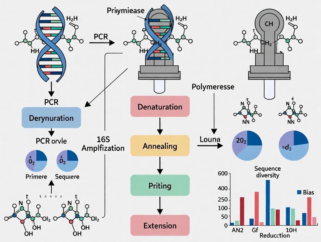
Strategies for Minimizing PCR Amplification Bias in 16S rRNA Sequencing: A Comprehensive Guide for Biomedical Researchers
PCR amplification is an integral but problematic step in 16S rRNA gene sequencing, introducing significant bias that distorts microbial community profiles and threatens the validity of scientific conclusions.
Strategies for Minimizing PCR Amplification Bias in 16S rRNA Sequencing: A Comprehensive Guide for Biomedical Researchers
Abstract
PCR amplification is an integral but problematic step in 16S rRNA gene sequencing, introducing significant bias that distorts microbial community profiles and threatens the validity of scientific conclusions. This article provides a comprehensive framework for researchers and drug development professionals to understand, quantify, and mitigate these biases. Covering foundational concepts through advanced validation techniques, we detail how factors including primer selection, PCR conditions, enzyme choice, and GC content affect amplification efficiency. We present optimized wet-lab protocols, computational correction models, and rigorous validation strategies using mock communities to ensure accurate representation of microbial abundances in diverse research and clinical applications.
Understanding the Sources and Impact of PCR Bias in 16S rRNA Studies
In 16S rRNA gene sequencing, Polymerase Chain Reaction (PCR) amplification is a critical step that can systematically distort the representation of microbial communities in your samples. These distortions, collectively known as PCR amplification bias, can be categorized into two primary sources based on their underlying mechanisms. Primer-mismatch bias originates from incomplete complementarity between the primer and template DNA, primarily affecting the initial PCR cycles. In contrast, non-primer-mismatch bias (PCR NPM-bias) arises from factors such as template GC content, amplicon length, and secondary structures, which influence amplification efficiency throughout all PCR cycles. Understanding this distinction is fundamental to designing robust experiments and implementing appropriate corrective strategies for accurate microbial community analysis [1] [2].
Defining the Bias: Mechanisms and Key Differences
Primer-Mismatch Bias
This form of bias occurs when sequences in the primer binding sites of the template DNA are not perfectly complementary to the primers used in the amplification reaction.
- Mechanism: A mismatch, particularly near the 3' end of the primer, reduces the efficiency with which the DNA polymerase can extend the primer. This leads to preferential amplification of templates with perfectly matching sequences.
- Phase of PCR Impacted: This bias is introduced almost exclusively during the first three cycles of PCR. After these initial cycles, the original primer-binding sequence on the template is replaced by a sequence that is perfectly complementary to the primer, effectively eliminating the mismatch in subsequent cycles [1] [2].
- Impact: One study demonstrated that a single mismatch in a universal bacterial primer could lead to an almost exponential increase in preferential amplification as the annealing temperature was raised from 47°C to 61°C [3]. This can cause the under-representation or complete dropout of specific taxa from your community profile.
Non-Primer-Mismatch Bias (PCR NPM-bias)
This bias stems from the physicochemical properties of the DNA template itself and the kinetics of the PCR process, independent of primer binding.
- Mechanism: Factors such as GC content, secondary structures, and overall template complexity can affect the denaturation and elongation efficiency during each PCR cycle. For example, GC-rich templates are harder to denature, leading to lower amplification efficiency [4].
- Phase of PCR Impacted: This bias operates throughout all cycles of the PCR reaction, from the mid-cycles (e.g., cycles 10-35) all the way to the late stages [1] [5].
- Impact: PCR NPM-bias can skew estimates of microbial relative abundances by a factor of 4 or more, significantly misrepresenting the true structure of the community [1]. One investigation found that as few as ten PCR cycles could deplete loci with a GC content >65% to about 1/100th of the mid-GC reference loci [4].
The following diagram illustrates the temporal dynamics and primary causes of these two distinct bias types during a typical PCR process.
The following table summarizes the core characteristics of both bias types, highlighting their distinct causes, impacts, and mitigation strategies.
| Feature | Primer-Mismatch Bias | Non-Primer-Mismatch Bias (NPM-Bias) |
|---|---|---|
| Primary Cause | Incomplete complementarity between primer and template DNA sequence [2] [3]. | Template GC content, secondary structure, and PCR stochasticity [1] [4]. |
| Key Mechanism | Reduced primer annealing and extension efficiency due to mismatches, especially at the 3' end [3]. | Incomplete denaturation of GC-rich templates and differential amplification efficiency per cycle [4]. |
| Phase of PCR | First 3 cycles [1]. | All cycles, with significant effects in mid-to-late cycles (cycles 10-35) [1] [5]. |
| Major Impact | Preferential amplification of perfect-match templates; failure to amplify taxa [2]. | Skewing of relative abundances by a factor of 4 or more [1]. |
| Primary Mitigation | Use of degenerate primers; lower annealing temperature; PEX-PCR method [2] [3]. | Use of PCR enhancers (e.g., betaine); optimized thermocycling; computational correction [1] [4]. |
Troubleshooting Guide & FAQs
Frequently Asked Questions
Q1: My negative controls are clean, but my low-biomass samples show high variability in rare species. What could be the cause? A: This is a classic sign of PCR stochasticity, a form of NPM-bias. In early PCR cycles, the random amplification of a limited number of starting DNA molecules can dramatically skew representation. This is particularly pronounced in low-biomass samples where template copies are scarce. To mitigate this, you can:
- Increase template input where possible.
- Perform technical replicates to identify and average out stochastic effects.
- Use a mock community as a positive control to quantify this variability [5] [6].
Q2: I am using well-established, "universal" primers, but I suspect I am missing certain archaeal groups. What type of bias is this likely to be? A: This is most likely primer-mismatch bias. Even "universal" primers may have mismatches to specific, often under-represented, taxonomic groups. For example, it was found that adding degeneracy to the 515F primer helped remove biases against Crenarchaeota/Thaumarchaeota [7]. To address this:
- Review the literature for primer updates targeting your missed groups.
- Consider using a primer pool with higher degeneracy.
- Lower the annealing temperature slightly to allow for some mismatch tolerance, though this may reduce specificity [3] [7].
Q3: My sequencing data under-represents GC-rich organisms despite using a validated protocol. How can I confirm and fix this NPM-bias? A: You can confirm this by running a qPCR bias assay on a panel of GC-varied amplicons [4]. To fix it, focus on wet-lab optimizations:
- Add PCR enhancers like betaine (1-2 M) or DMSO to lower strand separation temperatures.
- Optimize thermocycling conditions by extending denaturation times (e.g., from 10 s to 80 s per cycle) to ensure complete denaturation of GC-rich templates.
- Evaluate different polymerase blends known for better performance on complex templates [8] [4].
Experimental Protocol: PEX-PCR for Reducing Primer-Mismatch Bias
The Polymerase-exonuclease (PEX) PCR method is a novel strategy that separates the primer-template and primer-amplicon interactions to minimize biases from degenerate primer pools and primer-template mismatches [2].
Workflow Summary:
- Initial Limited-Cycle PCR: Perform a small number of PCR cycles (e.g., 3-5) using your degenerate primer pool and genomic DNA template.
- Exonuclease Digestion: Treat the product with an exonuclease to degrade the remaining primers from the first PCR. This step can often be performed without a reaction cleanup.
- Second PCR Amplification: Use a fresh, non-degenerate primer set (lacking the original degeneracies) to amplify the products from the first PCR for the remaining cycles.
Key Advantage: This method allows the initial primer binding to occur under low-stringency conditions if needed, reducing the impact of mismatches. The subsequent amplification with uniform primers ensures that all templates are amplified with equal efficiency in the later stages, substantially improving the evenness of sequence recovery from mock communities [2].
The Scientist's Toolkit: Research Reagent Solutions
The following table lists key reagents and their specific roles in mitigating different types of PCR bias in 16S rRNA gene sequencing.
| Reagent / Tool | Function / Mechanism | Relevant Bias |
|---|---|---|
| Betaine | Reduces melting temperature differences; equalizes amplification efficiency of GC-rich and AT-rich templates by acting as a destabilizer [8] [4]. | Non-Primer-Mismatch (GC Bias) |
| DMSO | Disrupts base pairing, helping to denature secondary structures and lower the melting temperature of DNA [8]. | Non-Primer-Mismatch (GC Bias) |
| PEX-PCR Method | Separates primer-template and primer-amplicon interactions; reduces bias from primer degeneracies and mismatches [2]. | Primer-Mismatch |
| Q5 Hot Start High-Fidelity Master Mix | A premixed mastermix that provides high fidelity and robust performance, reducing manual handling errors and batch effects [6]. | General Protocol Variability |
| AccuPrime Taq HiFi Blend | An alternative polymerase blend shown to amplify sequencing libraries more evenly than some standard enzymes [4]. | Non-Primer-Mismatch |
| Degenerate Primers (e.g., 515F-Y/806R) | Primer pools with added degeneracy to cover sequence variants, improving the detection of specific taxa like Crenarchaeota and SAR11 [7]. | Primer-Mismatch |
Computational Correction of PCR Bias
For biases that cannot be fully eliminated experimentally, computational post-processing offers a solution. A prominent approach involves using log-ratio linear models to correct for PCR NPM-bias [1].
Conceptual Framework: This model builds on the principle that each cycle of PCR amplifies each template with a taxon-specific efficiency. If the true ratio of two taxa prior to PCR is A/B, then after x cycles, the ratio becomes A/B × (EA/EB)x, where E is the per-cycle amplification efficiency.
Implementation: By using calibration data (e.g., from mock communities) or Bayesian modeling techniques applied to sample data, these efficiency ratios can be estimated. The observed sequencing data can then be transformed to estimate the true relative abundances before amplification, thereby correcting for the systematic bias introduced during PCR [1]. This method is particularly powerful because it can mitigate bias even after data collection, though it requires careful statistical implementation.
In 16S rRNA gene sequencing, Polymerase Chain Reaction (PCR) amplification is an integral experimental step for profiling microbial communities. However, PCR is known to introduce multiple forms of bias, which can skew estimates of microbial relative abundances by a factor of four or more [9]. These biases impede accurate evaluation of community structure and present a substantial source of error in microbiome studies [9] [10]. Among the numerous sources of bias, primer specificity, GC-content, and amplicon length represent three critical and controllable factors. This guide provides troubleshooting advice and methodologies to identify, understand, and mitigate these key sources of amplification bias.
Frequently Asked Questions (FAQs)
General Bias Concepts
Q1: What is PCR amplification bias and why is it a problem in 16S sequencing? PCR amplification bias refers to the non-random, preferential amplification of some bacterial 16S rRNA gene templates over others during the PCR process. This bias is problematic because it distorts the true biological signal, causing the final sequencing data to misrepresent the actual abundance, diversity, and composition of the microbial community in the original sample. This can lead to incorrect conclusions in research and diagnostics [9] [11].
Q2: Are biases consistent and can they be corrected? Yes, a body of research suggests that PCR bias is often reproducible and predictable. Because the bias is partly induced by sequence composition, it is often similar in closely related taxonomic groups. This predictability allows for the development of computational correction factors and experimental calibration methods to mitigate its effects [9] [11].
Primer Specificity
Q3: How does primer specificity contribute to amplification bias? Primer specificity bias occurs due to sequence divergence in the primer binding sites on the 16S rRNA gene. Even single nucleotide mismatches between the primer and the template, especially near the 3' end, can lead to preferential amplification of up to 10-fold [9]. This means taxa with perfect matches to the primers will be overrepresented, while those with mismatches may be undetected or severely underrepresented [9] [10] [11].
Q4: What are the best practices for selecting and designing primers to minimize bias?
- Use Degenerate Primers: Incorporate degenerate bases at variable positions to account for sequence diversity, which can broaden taxonomic coverage and reduce bias [11] [12].
- Optimize for Coverage and Efficiency: Utilize computational tools like mopo16S or Primer-BLAST to design primers that simultaneously maximize coverage (the fraction of bacterial sequences targeted), efficiency (predictable PCR performance), and minimize matching-bias (differences in how many primers bind to each taxon) [12].
- Validate Experimentally: Always test primer pairs on mock communities of known composition to assess their performance and potential biases for your specific sample type [10].
GC-Content
Q5: How does template GC-content cause amplification bias? Templates with very low or very high GC-content amplify less efficiently than those with moderate GC-content. This is because low GC-content sequences form less stable duplexes, while high GC-content sequences can form stable secondary structures that impede polymerase progression, leading to their under-representation in the final sequencing library [11] [12].
Q6: What is the optimal GC-content for PCR primers? For reliable amplification, primers should have a GC-content generally between 40%–60% [12] [13]. A "GC clamp" (one or two G or C bases at the 3' end) can promote stable binding, but avoid more than 3 G/C in the final five bases to prevent non-specific priming [13].
Amplicon Length
Q7: Why does amplicon length matter for amplification bias? Amplicon length influences bias in two primary ways:
- Amplification Efficiency: During PCR, shorter sequences are often amplified preferentially over longer ones. Furthermore, in samples with degraded DNA (e.g., from formalin-fixed tissues or processed foods), longer amplicons may fail to amplify altogether, leading to false negatives [11] [14].
- Viability qPCR (v-qPCR) Specificity: In techniques like v-qPCR that use dyes to distinguish live/dead cells, longer amplicons increase the probability of dye binding and effectively blocking amplification of DNA from dead cells. However, this comes at the cost of overall PCR efficiency [15].
Q8: Is there an optimal amplicon length to minimize bias? The "optimal" length is a trade-off and depends on the application:
- For standard 16S rRNA gene sequencing, shorter amplicons (e.g., single variable regions like V4) can reduce length-dependent bias and are compatible with short-read sequencing. However, longer amplicons (e.g., full-length 16S) can provide superior taxonomic resolution [10] [16].
- For v-qPCR, a range of ~200-400 bp is suggested as a working compromise, providing good live/dead distinction while maintaining reasonable PCR efficiency [15].
- For highly degraded DNA, amplicons of 50-80 bp are crucial for successful detection and to avoid false negatives [14].
Troubleshooting Guides
| Symptom in Data | Potential Cause | Next Steps for Verification |
|---|---|---|
| Systematic under-representation of a specific phylum (e.g., Bacteroidetes). | Primer mismatch due to poor binding site conservation. | Check in silico coverage of your primers against a database like SILVA. Compare with a different primer set. |
| Poor representation of taxa with very high or very low GC genomes. | GC-content bias. | Analyze the GC-content of under-represented taxa. Use PCR additives like DMSO or betaine in optimization. |
| Low library diversity or failure to amplify in samples with degraded DNA. | Amplicon length is too long for the template. | Re-attempt PCR with a shorter amplicon target. Check DNA quality via bioanalyzer. |
| Inconsistent community profiles between technical replicates. | PCR drift due to stochastic early-cycle amplification. | Reduce PCR cycle number and/or pool multiple PCR replicates [6]. |
Guide 2: Experimental Protocols for Mitigation
Protocol 1: A Paired Experimental and Computational Approach to Measure PCR NPM-Bias This protocol allows you to measure and correct for non-primer-mismatch (NPM) bias directly from your samples [9].
- Create a Calibration Sample: Pool aliquots of extracted DNA from all study samples.
- Generate Cycle Series: Split the pooled sample and amplify aliquots for different numbers of PCR cycles (e.g., 15, 20, 25, 30 cycles).
- Sequence and Model: Sequence all aliquots and use a log-ratio linear model (e.g., with the
fidoR package) to relate the observed composition to the PCR cycle number. - Apply Correction: The intercept of this model estimates the sample's composition prior to PCR NPM-bias, allowing for computational correction of your study data.
Protocol 2: Optimizing Amplicon Length for v-qPCR This method helps determine the optimal amplicon length for viability qPCR [15].
- Design Multiple Primer Sets: Design several primer sets targeting incrementally increasing amplicon lengths (e.g., from 68 bp to 906 bp) for your target organism.
- Treat with PMA: Split a sample of your bacteria into live and heat-killed portions, treating both with a viability dye (PMA).
- Run qPCR: Perform qPCR on both live and killed samples using all primer sets.
- Calculate ΔCq: For each amplicon length, calculate the difference in quantification cycle (ΔCq) between live and killed cells.
- Identify Optimal Range: Plot ΔCq against amplicon length. The optimal range is where ΔCq is high (good live/dead distinction) while maintaining acceptable PCR efficiency (minimal Cq increase in live samples). This typically falls between 200-400 bp [15].
Table 1: The Trade-off Between Amplicon Length, Live/Dead Distinction, and PCR Efficiency in v-qPCR [15]
| Bacterium | Minimum Amplicon Length (bp) for ~79% of Max ΔCq | ΔCq at Minimum Length | Maximum Amplicon Length (bp) for ~98.5% of Max ΔCq | ΔCq at Maximum Length |
|---|---|---|---|---|
| A. actinomycetemcomitans | 200 - 224 | 16.1 - 16.2 | 355 - 403 | 20.1 - 20.3 |
| P. intermedia | 227 | 18.3 | 414 | 22.9 |
| F. nucleatum | 156 | 12.6 | 278 | 15.7 |
| E. coli | 201 | 14.4 | 380 | 18.0 |
| General Guideline | ~200 bp | Good distinction | ~400 bp | Max distinction, lower efficiency |
Table 2: Impact of Short Amplicons on Detectability in Challenging Samples [14]
| Sample Type | Target | Short Amplicon Result (50-80 bp) | Long Amplicon Result (86-170 bp) |
|---|---|---|---|
| Soybean Oil | Lectin gene | Detected (Ct = 29) | Detected with higher Ct (Ct = 38) |
| Peanut Oil | Arah gene | Detected (Ct = 31) | No Amplification |
| Rapeseed Oil | CruA gene | Detected (Ct = 34) | No Amplification |
Workflow Diagrams
Diagram 1: Workflow for measuring and correcting PCR NPM-bias using a calibration experiment.
Diagram 2: Process for determining the optimal amplicon length for a v-qPCR assay.
The Scientist's Toolkit: Research Reagent Solutions
Table 3: Essential Materials and Reagents for Bias Mitigation
| Item | Function & Rationale | Example / Specification |
|---|---|---|
| Mock Community Standards | Positive control with known composition to quantify primer bias and bioinformatic pipeline performance. | ZymoBIOMICS Microbial Community Standards (D6300, D6331) [10] [16] |
| Spike-in Controls | Internal standards added to samples to convert relative abundance data to absolute abundance. | ZymoBIOMICS Spike-in Control I (D6320) [16] |
| High-Fidelity Polymerase | Reduces PCR-introduced errors and can improve amplification uniformity of complex mixtures. | Q5 Hot Start High-Fidelity Master Mix [6] |
| PCR Additives | Helps ameliorate biases from GC-content and secondary structures. | DMSO, Betaine |
| Viability Dyes (PMA/EMA) | Suppresses amplification of DNA from membrane-compromised (dead) cells in v-qPCR. | Propidium Monoazide (PMA) [15] |
| Primer Design Software | Computationally optimizes primers for coverage, specificity, and efficiency before synthesis. | NCBI Primer-BLAST, mopo16S, DegePrime [12] |
The Impact of PCR Cycle Number on Community Representation and Diversity
Frequently Asked Questions (FAQs)
Q1: How does increasing the PCR cycle number impact the sequencing of low microbial biomass samples? Increasing the PCR cycle number is a common strategy to improve sequencing coverage for low microbial biomass samples (e.g., blood, milk, tissue biopsies). While higher cycles (e.g., 35-40) significantly increase the number of usable sequences, they do not necessarily alter core ecological metrics like alpha-diversity or beta-diversity patterns compared to lower cycle numbers (e.g., 25). This allows for the successful profiling of samples that would otherwise yield uninterpretable data due to low coverage [17].
Q2: What is PCR amplification bias and how does it relate to cycle number? PCR amplification bias refers to the distortion of true microbial abundances because different DNA templates are amplified with varying efficiencies. This bias can skew estimates of microbial relative abundances by a factor of 4 or more. During mid-to-late stage PCR cycles, this bias becomes increasingly pronounced as templates with higher amplification efficiencies out-compete others, making cycle number a critical parameter to control [9].
Q3: Can I reduce the number of PCR replicates to save on costs and time? Yes, for standard 16S rRNA gene sequencing, evidence suggests that pooling multiple PCR amplifications per sample (a common practice to reduce PCR drift) may not be necessary. Studies have found no significant difference in high-quality read counts, alpha diversity, or beta diversity between libraries prepared from single, duplicate, or triplicate PCR reactions. This can streamline your protocol and reduce reagent use [6].
Q4: What is a major cause of failed 16S rRNA sequencing in human-derived samples? A major issue is off-target amplification of human DNA, particularly when using primers for the V4 region of the 16S rRNA gene. In human biopsy samples, this can lead to an average of 70% of sequenced reads aligning to the human genome instead of bacterial targets. Switching to optimized primers targeting the V1-V2 region can drastically reduce this problem and improve taxonomic resolution [18].
Troubleshooting Guides
Problem: Low Library Yield or No Amplification from Low Biomass Samples
This is a common issue when working with samples containing low bacterial DNA, such as blood, milk, or sterile tissues.
| Possible Cause | Recommended Solution |
|---|---|
| Insufficient PCR cycles | For low biomass samples, increase the PCR cycle number to 35 or 40 cycles to enhance detection probability [17]. |
| Inhibitors in DNA template | Re-purify the DNA sample using bead-based or column-based cleanups to remove salts, phenols, or other contaminants [19]. |
| Suboptimal primer selection | If working with human-associated samples, use primers less prone to off-target human DNA amplification (e.g., V1-V2 primers instead of V4) [18]. |
| Inaccurate DNA quantification | Use fluorometric methods (e.g., Qubit) rather than UV absorbance for quantifying input DNA, as the latter can overestimate usable concentration [19]. |
Problem: Over-Amplification Artifacts and Bias
Excessive PCR cycling can introduce artifacts and bias, even while improving coverage.
| Possible Cause | Recommended Solution |
|---|---|
| Too many PCR cycles | For high-biomass samples (e.g., stool, soil), limit cycles to 25-30 to minimize over-amplification artifacts and bias. For low-biomass samples, balance the need for coverage with the potential for increased chimeras [17] [20]. |
| High-fidelity polymerase error | Use a high-fidelity DNA polymerase and ensure balanced dNTP concentrations to reduce sequencing errors introduced during amplification [21] [22]. |
| Chimera formation | Implement a robust chimera detection and removal step in your bioinformatics pipeline (e.g., using Uchime). Chimera rates can be as high as 8% in raw reads [20]. |
Experimental Data and Protocols
Quantitative Impact of PCR Cycle Number
The following table summarizes key findings from a study that directly evaluated the effect of PCR cycle number on 16S rRNA sequencing results from low-biomass samples [17].
| Sample Type | PCR Cycles Tested | Impact on Coverage | Impact on Alpha & Beta Diversity |
|---|---|---|---|
| Bovine Milk | 25, 30, 35, 40 | Significantly increased with higher cycles | No significant differences detected |
| Murine Pelage | 25, 40 | Significantly increased with higher cycles | No significant differences detected |
| Murine Blood | 25, 40 | Significantly increased with higher cycles | No significant differences detected |
Detailed Protocol: Mitigating Bias via a Calibration Experiment
This protocol, based on contemporary research, allows for the measurement and correction of PCR bias without relying on mock communities [9].
Objective: To computationally correct for non-primer-mismatch PCR bias (NPM-bias) in microbiota datasets.
Workflow Steps:
- Create a Calibration Sample: Prior to PCR, pool aliquots of extracted DNA from every study sample into a single, representative pooled sample.
- Generate Calibration Curve: Split the pooled sample into several aliquots. Amplify each aliquot for a different number of PCR cycles (e.g., 10, 15, 20, 25, 30), covering a wide range.
- Sequence All Samples: Sequence the calibration aliquots alongside your main study samples, which are all amplified with a standard cycle number.
- Computational Correction: Use a log-ratio linear model (e.g., with the
fidoR package) to analyze the calibration data. The model infers the original sample composition (intercept) and the taxon-specific amplification efficiencies (slope) to correct the bias in the main study data.
Below is a workflow diagram of this calibration experiment:
The Scientist's Toolkit: Essential Research Reagents
| Item | Function & Rationale |
|---|---|
| High-Fidelity Hot-Start Polymerase (e.g., Q5, Phusion) | Reduces non-specific amplification and errors during the initial PCR cycles, improving specificity and yield [6] [22]. |
| Droplet Digital PCR (ddPCR) | Provides absolute quantification of bacterial load and initial community ratios without amplification bias, serving as a gold standard for validating NGS data and bias correction models [23]. |
| Mock Microbial Community | A DNA mixture of known bacterial composition. It is essential for validating your entire workflow, quantifying batch effects, and estimating error rates [23] [20]. |
| Bead-Based Cleanup Kits (e.g., AMPure XP) | Used for consistent purification and size-selection of PCR products, effectively removing primer dimers and other unwanted artifacts [17] [6]. |
| Optimized Primer Sets (e.g., for V1-V2) | Primer pairs designed to minimize off-target amplification (e.g., of human host DNA) are crucial for successful sequencing of host-derived samples like biopsies [18]. |
How Genomic GC-Content Correlates with Amplification Efficiency
Frequently Asked Questions
What are the primary consequences of GC-content bias in 16S sequencing? GC-content bias leads to non-homogeneous amplification of template DNA, where some sequences are preferentially amplified over others. This results in skewed representation of microbial taxa in your final sequencing data, compromising the accuracy and sensitivity of both alpha and beta diversity analyses. Widely used metrics like Shannon diversity and Weighted-Unifrac are particularly sensitive to this bias [24].
My amplification of a GC-rich region has failed. What should I check first? Your initial troubleshooting should focus on three key areas:
- Polymerase Choice: Standard polymerases often stall at complex secondary structures. Switch to a polymerase specifically engineered for high GC content, such as OneTaq or Q5, which are often supplied with a specialized GC buffer and enhancer [25].
- Reaction Additives: Incorporate additives like DMSO, betaine, or formamide. These work by reducing secondary structure formation (e.g., hairpins) and increasing primer annealing stringency, which helps denature stable GC-rich templates [26] [27].
- Thermal Cycling Conditions: Optimize your annealing temperature. A higher temperature can improve specificity and help denature secondary structures. Also, consider using a 2-step PCR protocol or a "slowdown PCR" method with adjusted ramp speeds to improve the amplification of long, GC-rich targets [27].
How can I predict if my target sequence will be difficult to amplify based on its sequence? While overall GC content is a good initial indicator, regionalized GC content is a much more powerful predictor. Research has shown that calculating GC content within a sliding window (e.g., 21 bp) and identifying regions that exceed a threshold (e.g., 61% GC) significantly improves the ability to predict PCR success. Templates with high localized GC regions are far more challenging to amplify than those with evenly distributed GC content [28].
Are there ways to correct for GC bias bioinformatically after sequencing? Yes, bioinformatic normalization approaches can help correct sequencing biases. Tools like FastQC and Picard can first help you identify and quantify the level of GC bias in your data. Subsequent bioinformatic algorithms can then adjust read depth based on local GC content, improving coverage uniformity and the accuracy of downstream analyses like variant calling [29].
GC Content as a Predictor of PCR Efficiency
The following table summarizes key quantitative findings on the relationship between template GC characteristics and PCR amplification success.
| GC Characteristic | Impact on Amplification Efficiency | Experimental Context | Key Finding |
|---|---|---|---|
| Overall GC Content >60% | Major challenge; often leads to failed amplification or low yield [25] [26] | Amplification of nicotinic acetylcholine receptor subunits (GC=58-65%) [26] | Requires optimized protocols with additives and specialized polymerases. |
| Regionalized GC >61% | Stronger predictor of failure than overall GC content [28] | Amplification of 1,438 human exons [28] | Improved specificity (84.3%) and sensitivity (94.8%) in predicting PCR outcome. |
| Local GC-rich stretches | Forms stable secondary structures (hairpins), blocking polymerase [27] | Amplification of Mycobacterium bovis gene Mb0129 (77.5% GC) [27] | Causes severe drop-off in efficiency; necessitates specialized cycling conditions. |
| Progressive Skewing | A small subset (~2%) of sequences can have efficiencies as low as 80% relative to the mean [30] | Multi-template PCR on 12,000 synthetic DNA sequences [30] | Leads to drastic under-representation after as few as 30 PCR cycles. |
Experimental Protocols for Mitigating GC-Bias
Protocol 1: Optimized Workflow for GC-Rich Amplicons
This workflow is designed for amplifying difficult, GC-rich targets, such as those encountered in 16S rRNA gene sequencing.
Detailed Steps:
- Polymerase and Buffer System: Replace standard Taq polymerase with a high-fidelity enzyme engineered for GC-rich templates, such as Q5 or OneTaq DNA Polymerase. Use the specialized GC buffer and GC enhancer supplied with these systems. The enhancer typically contains a proprietary mix of additives that lower the melting temperature of DNA and disrupt secondary structures [25].
- Additive Optimization: If further optimization is needed, test the addition of 1-10% DMSO or 0.5 M to 2.5 M betaine to the reaction mix. These compounds are known to equalize the melting temperatures of DNA, preventing the formation of secondary structures like hairpins and improving the yield of GC-rich amplicons [26] [27].
- Mg2+ Concentration: Set up a reaction series testing MgCl2 concentrations in 0.5 mM increments from 1.0 mM to 4.0 mM. Magnesium is a critical cofactor for polymerase activity, and its optimal concentration can vary significantly for difficult templates [25].
- Thermal Cycling Parameters:
- Annealing Temperature: Perform a temperature gradient PCR to determine the optimal annealing temperature (Ta). A higher Ta (e.g., 5°C higher than the calculated Tm) can significantly improve specificity by preventing non-specific primer binding [25].
- Advanced Cycling: For particularly long (>1 kb) or difficult targets, employ a 2-step PCR protocol that combines annealing and extension at a higher temperature (e.g., 68°C). Using a thermal cycler with adjustable ramp speed and setting it to a slower speed (e.g., 1-2°C/second) can dramatically improve success rates by allowing more time for the polymerase to unwind and replicate highly structured DNA [27].
Protocol 2: Validating Primer Efficiency for Quantitative Analysis
For applications like qPCR, ensuring uniform and high amplification efficiency is critical for accurate quantification. This protocol ensures primers meet strict efficiency standards before use in 16S sequencing studies [31].
Procedure:
- Sequence-Specific Primer Design: For each target gene (e.g., a 16S rRNA hypervariable region), retrieve all homologous sequences. Design primers based on single-nucleotide polymorphisms (SNPs) unique to the target to ensure specificity and avoid co-amplification of closely related sequences.
- Generate a Standard Curve: Using a serial dilution (e.g., 1:10) of your template cDNA, run a qPCR assay for each primer pair.
- Calculate Efficiency and R²: Plot the log of the template concentration against the Ct value for each dilution. Perform linear regression analysis. The slope of the line is used to calculate the amplification efficiency (E) using the formula: ( E = 10^{(-1/slope)} - 1 ). An ideal primer pair will have an efficiency (E) of 100% ± 5% and a correlation coefficient (R²) ≥ 0.9999 [31].
- Validation: Only primer pairs that meet these stringent criteria should be used for subsequent quantitative experiments to ensure that observed abundance differences reflect biology and not technical bias.
The Scientist's Toolkit: Essential Reagents for GC-Rich PCR
| Reagent Category | Example Products | Function in GC-Rich PCR |
|---|---|---|
| Specialized Polymerases | Q5 High-Fidelity DNA Polymerase, OneTaq DNA Polymerase [25] | Engineered to resist stalling at stable secondary structures; often supplied with proprietary GC buffers. |
| PCR Enhancers/Additives | Betaine, DMSO, Formamide [26] [27] | Disrupt hydrogen bonding, lower DNA melting temperature, and prevent secondary structure formation. |
| GC-Enhanced Master Mixes | OneTaq Hot Start 2X Master Mix with GC Buffer, Q5 High-Fidelity 2X Master Mix [25] | Pre-mixed convenience with optimized buffer/enhancer formulations for robust amplification of difficult targets. |
| Magnesium Salts (MgCl₂) | Supplied with polymerase buffers | A critical cofactor; fine-tuning its concentration (1.0-4.0 mM) is essential for polymerase activity and primer annealing in GC-rich contexts [25]. |
FAQ: Understanding and Troubleshooting PCR Bias in 16S Sequencing
What are the primary consequences of PCR amplification bias in my 16S rRNA data?
PCR amplification bias systematically distorts your data in two key ways:
- Skewed Abundance Estimates: The relative proportions of organisms in your data no longer accurately reflect their true ratios in the original sample. This bias can skew estimates of microbial relative abundances by a factor of 4 or more [32] [33]. This means a microbe representing 10% of the actual community could appear as either 40% or 2.5% in your results.
- Generation of Spurious OTUs: Bias can create artificial diversity. Chimeric sequences formed during PCR [34] and the differential amplification of intragenomic 16S gene copies [35] can be misinterpreted as unique Operational Taxonomic Units (OTUs), inflating diversity metrics and leading to false biological discoveries.
Why does my amplicon data show high levels of an archaeon (likeMethanobrevibacter) that doesn't match my biological expectations?
This is a classic sign of amplification bias, often caused by extensive length polymorphisms in the target gene region [36]. In a mixed community, templates with shorter amplicon lengths will amplify more efficiently than longer ones, especially when the sample DNA is fragmented (common in ancient or low-quality samples). If a particular organism's 16S gene is shorter for your chosen primer set, it will be disproportionately over-represented in your final data [36].
My sequencing library yield is low, and my electropherogram shows a sharp peak at ~70-90 bp. What is wrong?
A sharp peak at 70-90 bp is a clear indicator of adapter dimer contamination [19]. This occurs during library preparation due to:
- Inefficient Ligation: Poor ligase performance or suboptimal reaction conditions.
- Adapter-to-Insert Molar Imbalance: An excess of adapters in the reaction promotes adapter-dimer formation.
- Inadequate Purification: Failure to effectively remove these small artifacts after library construction [19]. These dimers consume sequencing resources and can result in low yields of usable data. You should re-optimize your ligation protocol and ensure a thorough cleanup with size selection.
How much can the DNA extraction protocol alone impact my microbial community profiles?
The choice of DNA extraction kit is one of the most significant sources of bias. Studies have shown that using different kits on the same mock community can lead to dramatically different results [37]. One kit might increase the observed proportion of Enterococcus by 50% while suppressing other genera, compared to another kit [37]. The bias introduced by DNA extraction is often much larger than that introduced by sequencing and classification [37].
Quantifying the Impact: Data on Bias Magnitude
The following table summarizes quantitative findings on the magnitude of bias from key studies.
Table 1: Documented Magnitude of PCR and Sample Preparation Biases
| Source of Bias | Observed Impact | Experimental Context |
|---|---|---|
| PCR (NPM-bias) | Skewed abundance estimates by a factor of 4 or more [32]. | Mock bacterial communities and human gut microbiota. |
| DNA Extraction | Error rates from bias of over 85% in some samples; technical variation was less than 5% for most bacteria [37]. | 80 mock communities comprised of seven vaginally-relevant bacterial strains. |
| Template Concentration | A significant impact on sample profile variability; low concentration (0.1-ng) templates showed higher variability [38]. | Soil and fecal DNA extracts sequenced on Illumina MiSeq. |
Experimental Protocols for Bias Characterization
Protocol 1: Using Mock Communities to Quantify Total Bias
This protocol allows you to quantify the total bias introduced by your entire sample processing pipeline [37].
- Select Bacterial Strains: Decide on a small subset of bacteria relevant to your study that can be cultured.
- Generate Experimental Design: Create a D-optimal mixture design with prescribed proportions for the mock communities. Include replicate runs to estimate pure error variance.
- Prepare Mock Communities: Grow each isolate to exponential phase and determine cell density. Combine the bacteria in the prescribed proportions to create the mock community samples.
- Process Samples: Subject the mock communities to your standard pipeline: DNA extraction, PCR amplification, sequencing, and taxonomic classification.
- Analyze Data: Compare the observed proportions from sequencing with the known, prescribed proportions from the experimental design. The difference is your total measured bias.
Protocol 2: Paired Modeling to Mitigate PCR NPM-Bias
This approach uses a statistical model to correct for non-primer-mismatch (NPM) PCR bias [32].
- Generate Standard Curves: Create a dilution series of a mock community with known composition. Include this as a standard in every sequencing run.
- Sequence Standards and Samples: Process both the mock community standards and your environmental samples (e.g., human gut microbiota) using the same 16S rRNA gene sequencing protocol.
- Model the Bias: Use the data from the mock standard to fit a log-ratio linear model. This model characterizes the relationship between the true relative abundances (known from the mock) and the observed relative abundances (from sequencing).
- Apply the Correction: Use the fitted model to predict and correct the true microbial relative abundances in your environmental samples based on your observed data [32].
Research Reagent Solutions for Bias Mitigation
Table 2: Key Reagents and Their Roles in Managing 16S Sequencing Bias
| Reagent / Tool | Function / Rationale | Example |
|---|---|---|
| Mock Communities | Ground-truthing for quantifying bias introduced by the entire wet-lab workflow [37]. | Defined mixtures of cultured bacterial strains (e.g., 7 vaginally-relevant species) [37]. |
| High-Fidelity Polymerase | Reduces PCR errors and chimera formation during amplification. | LongAmp Taq MasterMix (used in full-length 16S protocols) [34]. |
| Emulsion (Micelle) PCR | Physically separates template molecules to prevent chimera formation and PCR competition, enabling absolute quantification [34]. | micPCR protocol for full-length 16S rRNA gene amplification [34]. |
| Full-Length 16S Primers | Provides superior taxonomic resolution compared to short variable regions, helping to resolve species and strains [35] [34]. | Primers 16SV1-V9F and 16SV1-V9R [34]. |
| Internal Calibrator (IC) | Allows for absolute quantification of 16S rRNA gene copies, enabling subtraction of background contaminating DNA [34]. | Synechococcus 16S rRNA gene copies added to each sample [34]. |
| Barcoded Primers | Enables multiplex sequencing of multiple samples, reducing inter-lane sequencing variability [38]. | Unique barcodes for each sample, part of the cDNA-PCR sequencing kit (ONT) [34]. |
Workflow Diagrams
PCR Bias Consequences and Mitigation
Experimental Protocol for Bias Quantification
Practical Laboratory Protocols to Reduce Bias During Library Preparation
Frequently Asked Questions (FAQs)
Q1: Why do my "universal" 16S rRNA primers fail to detect all target microorganisms in my complex gut microbiome samples?
Even well-established "universal" primers cannot achieve 100% coverage of all microorganisms. In silico evaluations reveal that commonly used primers may miss tens of thousands of bacterial and archaeal species due to sequence mismatches in priming sites [39]. This limitation stems from unexpected variability even within traditionally conserved regions of the 16S rRNA gene [40]. For example, the widely used 515F-806R primer pair covers approximately 83.6% of bacteria and 83.5% of archaea but misses 62,406 bacterial species and 3,306 archaeal species [39]. This coverage gap becomes particularly problematic when studying specific taxa of interest that may be systematically underrepresented.
Q2: How does primer degeneracy improve coverage, and what are the practical limits for degeneracy in primer design?
Degenerate primers incorporate mixtures of similar sequences with different nucleotides at variable positions, enabling recognition of multiple genetic variants within microbial communities [41]. This approach significantly enhances coverage of diverse microorganisms, as demonstrated when Hugerth et al. increased archaeal coverage from 53% to 93% by changing one position in a primer from C to Y (C/T) [39]. However, practical guidelines recommend:
- Avoiding degeneracy in the last 3 nucleotides at the 3' end [41]
- Designing primers with less than 4-fold degeneracy at any single position [41]
- Beginning with a primer concentration of 0.2 µM and increasing in 0.25 µM increments if PCR efficiency is poor [41] Excessive degeneracy reduces the effective concentration of primer molecules complementary to any specific template and increases the risk of non-specific amplification [41].
Q3: Which 16S rRNA variable region provides the best taxonomic resolution for microbiome studies?
No single variable region can differentiate all bacteria, but some regions outperform others for specific applications. The table below summarizes the discriminatory power of different hypervariable regions based on in silico analysis:
Table 1: Performance Characteristics of 16S rRNA Variable Regions
| Target Region | Strengths | Limitations | Recommended Applications |
|---|---|---|---|
| V1-V3 | Good for Escherichia/Shigella; reasonable approximation of 16S diversity | Poor performance with Proteobacteria | General diversity surveys when full-length sequencing unavailable |
| V3-V5 | Suitable for Klebsiella | Poor classification of Actinobacteria | Targeted studies of specific pathogens |
| V4 | Most commonly used | Worst performance for species-level discrimination (56% fail accurate classification) | High-level taxonomic profiling |
| V6 | Distinguishes most bacterial species except enterobacteriaceae; differentiates CDC-defined select agents | Limited length for phylogenetic analysis | Diagnostic assays for specific pathogens |
| Full-length (V1-V9) | Highest taxonomic accuracy; enables species and strain-level discrimination | Requires third-generation sequencing platforms | Studies requiring maximum taxonomic resolution |
Sequencing the entire ~1500 bp 16S gene provides significantly better taxonomic resolution than any single sub-region, with nearly all sequences correctly classified to species level compared to substantial failure rates for sub-regions [35].
Q4: How can I computationally evaluate and improve the coverage of my custom primers?
The "Degenerate Primer 111" tool provides a user-friendly approach to enhance primer coverage by systematically adding degenerate bases to existing universal primers [39]. The workflow involves:
- Aligning your universal primer with the SSU rRNA gene of an uncovered target microorganism
- Iteratively generating a new primer that maximizes coverage for target microorganisms
- Maintaining or reducing coverage of non-target microorganisms This tool successfully modified eight pairs of universal primers, generating 29 new primers with increased coverage of specific targets [39]. Alternatively, the mopo16S software uses multi-objective optimization to simultaneously maximize efficiency, coverage, and minimize primer matching-bias [12].
Troubleshooting Guides
Problem: Inconsistent Microbial Community Profiles Between Technical Replicates
Potential Cause: PCR amplification bias from non-primer-mismatch sources (NPM-bias), which can skew estimates of microbial relative abundances by a factor of 4 or more [9].
Solution:
- Implement log-ratio linear models: These models can correct for NPM-bias by estimating relative amplification efficiencies across taxa [9]
- Standardize PCR conditions: Limit cycle numbers (typically 25-30 cycles) and maintain consistent template concentrations across replicates [9] [11]
- Use mock communities: Include control communities with known composition to quantify and correct for amplification biases [9]
Validation Experiment:
- Pool aliquots of extracted DNA from each study sample into a single calibration sample
- Split into aliquots and amplify for different PCR cycle numbers (e.g., 15, 20, 25, 30 cycles)
- Sequence all aliquots and apply log-ratio linear models to estimate pre-PCR composition [9]
Diagram 1: Workflow for PCR bias mitigation
Problem: Low Amplification Efficiency with Degenerate Primers
Potential Cause: Suboptimal primer design or PCR conditions that reduce annealing specificity, particularly problematic with highly degenerate primer mixtures where only a limited number of primer molecules complement the template [41].
Solution:
- Follow degenerate primer design guidelines:
- Place degenerate positions toward the 5' end rather than the 3' end
- Use Met- or Trp-encoding triplets at the 3' end when possible (these amino acids have single codons)
- Limit total degeneracy to avoid excessive sequence variety [41]
- Optimize PCR conditions:
- Increase primer concentration gradually from 0.2 µM to 0.45-0.7 µM if needed
- Adjust annealing temperature using gradient PCR
- Include betaine or DMSO to stabilize annealing when using highly degenerate primers
Validation Method: Test primer efficiency using in silico evaluation with TestPrime against the SILVA SSU database before wet-lab experimentation [39] [40]. Aim for ≥70% coverage across target phyla and ≥90% coverage for key genera of interest [40].
Problem: Inadequate Taxonomic Resolution at Species/Strain Level
Potential Cause: Short-read sequencing of limited variable regions provides insufficient phylogenetic information for fine-scale discrimination [35].
Solution:
- Transition to full-length 16S sequencing: Third-generation sequencing platforms (PacBio, Oxford Nanopore) enable sequencing of the entire ~1500 bp 16S gene, dramatically improving taxonomic resolution [35]
- Account for intragenomic variation: Bacterial genomes often contain multiple polymorphic 16S copies; properly resolving these variants can provide strain-level discrimination [35]
- Select optimal variable regions: If full-length sequencing is unavailable, choose variable regions based on your target taxa (see Table 1)
Experimental Design: For strain-level discrimination:
- Implement PacBio Circular Consensus Sequencing (CCS) with ≥10 passes to minimize errors
- Cluster sequences accounting for intragenomic 16S copy variants
- Validate putative strain-specific polymorphisms with complementary methods (e.g., qPCR, WGS)
Table 2: In silico Coverage of Selected Primer Pairs Across Dominant Gut Phyla
| Primer Set | Target Region | Actinobacteriota | Bacteroidota | Firmicutes | Proteobacteria | Overall Assessment |
|---|---|---|---|---|---|---|
| V3_P3 | V3 | 92% | 88% | 85% | 90% | High coverage across all phyla |
| V3_P7 | V3 | 90% | 86% | 82% | 88% | Balanced performance |
| V4_P10 | V4 | 85% | 92% | 80% | 83% | Strong for Bacteroidota |
| V1-V3_P5 | V1-V3 | 88% | 85% | 87% | 75% | Weak for Proteobacteria |
| V6-V8_P12 | V6-V8 | 82% | 80% | 90% | 85% | Strong for Firmicutes |
Note: Coverage percentages represent in silico amplification efficiency against SILVA database [40].
Research Reagent Solutions
Table 3: Essential Tools for Optimal Primer Design and Validation
| Resource | Type | Function | Key Features |
|---|---|---|---|
| SILVA SSU Ref NR | Database | Reference for in silico primer evaluation | 510,495 aligned rRNA sequences; TestPrime tool for coverage calculation [39] [40] |
| Degenerate Primer 111 | Software | Adding degenerate bases to existing primers | Iterative approach to maximize target coverage without increasing non-target amplification [39] |
| mopo16S | Algorithm | Multi-objective primer optimization | Maximizes efficiency, coverage, minimizes matching-bias; avoids degenerate primers [12] |
| FAS-DPD | Software | Family-specific degenerate primer design | Scores primers weighting 3' end conservation more heavily; works from protein alignments [42] |
| ZymoBIOMICS Gut Microbiome Standard | Mock Community | Experimental validation | 19 bacterial/archaeal strains with known 16S copy variation [40] |
| TestPrime | Online Tool | In silico primer evaluation | Calculates coverage against SILVA database with user-defined mismatch parameters [39] [40] |
Diagram 2: Primer selection decision tree
In 16S rRNA sequencing for microbiome research, the choice of polymerase chain reaction (PCR) enzyme is a critical experimental decision. PCR amplification bias, wherein some templates are amplified more efficiently than others, can significantly skew the representation of microbial communities, leading to erroneous biological conclusions. This technical support guide provides a detailed, evidence-based framework for selecting high-fidelity DNA polymerases to minimize these biases and ensure the accuracy and reliability of your 16S sequencing data.
FAQs and Troubleshooting Guides
FAQ 1: Why is polymerase fidelity critical for 16S rRNA sequencing?
PCR enzymes inherently incorporate errors during DNA amplification. In 16S sequencing, where community composition is inferred from sequence counts, these errors can create spurious sequences that are misinterpreted as novel taxa or rare biosphere members, artificially inflating diversity estimates [43] [20]. High-fidelity polymerases possess 3'→5' exonuclease (proofreading) activity, which allows them to identify and correct misincorporated nucleotides. This results in significantly lower error rates, preserving the true biological sequence and ensuring that the observed microbial diversity reflects the actual sample composition.
FAQ 2: How does PCR enzyme choice contribute to amplification bias?
Amplification bias occurs when DNA from different microbial taxa is amplified with varying efficiencies, distorting their true relative abundances. This bias can originate from several factors, including:
- Primer-Template Mismatches: Sequence variation in the primer-binding region across different taxa can lead to dramatic differences in amplification efficiency [9].
- Non-Primer-Mismatch (NPM) Bias: Even with perfect primer matches, differences in template properties (e.g., GC-content, secondary structure) can cause certain sequences to be amplified more efficiently than others throughout the PCR process [9].
- Enzyme Processivity: An enzyme's ability to synthesize long DNA fragments can vary, potentially biasing against longer amplicons.
One study demonstrated that PCR NPM-bias alone can skew estimates of microbial relative abundances by a factor of 4 or more [9]. High-fidelity enzymes, often paired with optimized buffers, can help mitigate these biases by providing more uniform amplification across diverse templates.
FAQ 3: What are the key performance metrics when comparing high-fidelity polymerases?
When selecting an enzyme for 16S sequencing, consider the following performance metrics, which are summarized in the table below:
- Fidelity (Error Rate): The frequency of misincorporated nucleotides, typically expressed as errors per base per duplication. Lower values are better.
- Processivity: The number of nucleotides a polymerase can incorporate in a single binding event, important for amplifying longer targets.
- Specificity: The ability to amplify only the intended target, minimizing non-specific products and primer-dimer formation. Hot-start enzymes are engineered to remain inactive at room temperature, greatly enhancing specificity [22] [44].
- Speed: The extension rate (e.g., seconds per kilobase), which can reduce overall cycling time.
- Inhibitor Tolerance: The enzyme's resistance to common PCR inhibitors found in sample types like soil or blood [22].
Table 1: Quantitative Comparison of DNA Polymerase Performance
| DNA Polymerase | Published Error Rate (Errors/bp/duplication) | Fidelity Relative to Taq | Proofreading Activity | Key Characteristics |
|---|---|---|---|---|
| Taq | ( 1 - 20 \times 10^{-5} ) [45] | 1x | No | Standard for routine PCR; lower cost but high error rate |
| Pfu | ( 1 - 2 \times 10^{-6} ) [45] | 6–10x better [45] | Yes | Classic high-fidelity enzyme |
| Phusion | (\sim 4.0 \times 10^{-7}) (HF buffer) [45] | >50x better [45] | Yes | High fidelity and fast extension time |
| Platinum SuperFi II | Not specified in data | >300x better [44] | Yes | Very high accuracy, suitable for complex cloning |
Troubleshooting Guide: Common PCR Issues in 16S Sequencing
Table 2: Troubleshooting Common PCR Problems in 16S Sequencing Workflows
| Observation | Possible Cause | Recommended Solution |
|---|---|---|
| Sequence Errors / High Error Rate | Low-fidelity polymerase | Use a high-fidelity, proofreading polymerase (e.g., Pfu, Phusion, Q5) [46]. |
| Suboptimal reaction conditions | Reduce the number of PCR cycles; decrease Mg2+ concentration; use fresh, balanced dNTPs [46]. | |
| No Product or Low Yield | Poor template quality or inhibitors | Re-purify template DNA; use polymerases with high inhibitor tolerance; add BSA [22] [47]. |
| Incorrect annealing temperature | Recalculate primer Tm and optimize annealing temperature using a gradient cycler [22] [48]. | |
| Insufficient polymerase | Increase the amount of polymerase or use an enzyme with higher sensitivity [22]. | |
| Non-Specific Bands / Multiple Bands | Lack of specificity / mispriming | Use a hot-start DNA polymerase to prevent activity at room temperature [44]. |
| Annealing temperature too low | Increase the annealing temperature stepwise [22]. | |
| Excess Mg2+ or primers | Optimize Mg2+ concentration; titrate primer concentrations (typically 0.1–1 µM) [22] [46]. | |
| Primer-Dimer Formation | Primer self-complementarity | Redesign primers to avoid 3'-end complementarity [48] [47]. |
| High primer concentration | Lower the primer concentration in the reaction [22]. |
Experimental Protocols
Protocol 1: Assessing PCR Amplification Bias Using a Mock Community
Purpose: To empirically quantify the amplification bias introduced by different PCR enzymes in your 16S sequencing pipeline.
Background: Using a mock microbial community with known, defined composition allows you to directly compare the sequencing results to the expected abundances, providing a ground truth for measuring bias [9] [43].
Materials:
- Mock Community: Genomic DNA from a defined set of bacterial strains (e.g., 20-30 strains from ZymoBIOMICS or ATCC).
- Test Polymerases: The high-fidelity enzymes you wish to compare (e.g., Q5, Phusion, Pfu).
- 16S rRNA Primers: Your standard primers targeting the V3-V4 or other hypervariable region.
- qPCR Instrument or Gel Electrophoresis System: For quantifying amplification efficiency.
Method:
- PCR Amplification: Amplify the mock community DNA in triplicate with each test polymerase, strictly controlling the number of cycles (e.g., 25-30 cycles) [22].
- Library Preparation and Sequencing: Prepare sequencing libraries from the amplified products and sequence on an Illumina MiSeq or similar platform.
- Bioinformatic Analysis: Process the raw sequencing data using your standard 16S pipeline (e.g., DADA2, QIIME2) to obtain Amplicon Sequence Variants (ASVs) or OTUs and their counts.
- Bias Calculation:
- Map the resulting ASVs to the known sequences of the mock community.
- For each taxon, calculate the Observed/Expected Ratio:
(Observed Read Count / Total Reads) / (Expected Genomic DNA Input / Total Input) - The variation in this ratio across taxa quantifies the bias introduced by each polymerase. An ideal enzyme would show a ratio close to 1 for all taxa.
The following workflow summarizes the experimental design for assessing PCR bias:
Protocol 2: A Paired Modeling and Experimental Approach to Mitigate Bias
Purpose: To measure and computationally correct for PCR NPM-bias directly from your experimental samples without a mock community.
Background: This method, adapted from [9], involves creating a calibration curve from your own samples to model how bias increases with PCR cycle number.
Method:
- Create Calibration Sample: Pool aliquots of extracted DNA from all study samples into a single calibration sample.
- Cycle Gradient PCR: Split the calibration sample into multiple aliquots. Amplify each aliquot for a different number of PCR cycles (e.g., 15, 20, 25, 30 cycles) using your chosen high-fidelity polymerase.
- Sequence and Model: Sequence all aliquots and use a log-ratio linear model (e.g., as implemented in the R package
fido) to analyze the data [9]. The model estimates the true starting composition (intercept) and the taxon-specific amplification efficiencies (slope). - Apply Correction: Use the fitted model to correct the bias in your main experimental dataset.
The Scientist's Toolkit: Research Reagent Solutions
Table 3: Essential Reagents for Minimizing PCR Bias in 16S Sequencing
| Reagent / Material | Function / Purpose | Key Considerations |
|---|---|---|
| High-Fidelity DNA Polymerase | Amplifies target DNA with minimal sequence errors. | Select enzymes with proofreading activity (e.g., Phusion, Q5, Pfu). Verify error rates from vendor data [45] [44]. |
| Mock Microbial Community | Provides a known standard for quantifying accuracy and bias. | Choose communities with complexity relevant to your sample type (e.g., HC227 for high complexity) [43]. |
| Hot-Start Polymerase | Prevents non-specific amplification and primer-dimer formation prior to the initial denaturation step. | Critical for improving specificity and yield in 16S PCR [44]. |
| PCR Additives (BSA, Betaine) | Enhances amplification of difficult templates (e.g., high GC-content) and mitigates effects of inhibitors. | BSA can bind inhibitors; betaine helps denature GC-rich secondary structures [22] [48]. |
| Gel Extraction / PCR Cleanup Kit | Purifies the target amplicon from non-specific products, primer-dimers, and unused reagents. | Essential for obtaining a clean library for sequencing. |
| Standardized 16S rRNA Primer Set | Ensures specific and uniform amplification of the target variable region. | Use well-validated, high-purity primers. Consider degenerate primers to reduce primer bias [11]. |
In 16S rRNA gene sequencing, the polymerase chain reaction (PCR) is a critical step for amplifying target genes from complex microbial communities. However, standard thermocycling conditions can introduce significant biases by preferentially amplifying certain bacterial templates over others, leading to a distorted view of the true microbial composition. This guide addresses how the precise control of denaturation time and ramp rates—often overlooked parameters—can be optimized to minimize these biases, thereby enhancing the accuracy and reproducibility of your microbiome research.
FAQ: Thermocycling and PCR Bias in 16S Sequencing
1. How does denaturation time specifically influence bias in 16S amplicon sequencing? Insufficient denaturation time can lead to incomplete separation of DNA strands, particularly for templates with high GC content or secondary structures. This results in inefficient primer binding and biased amplification of certain sequences in the community. Overly long denaturation times, however, can reduce polymerase activity over many cycles, also skewing results [19] [22]. The goal is to use the minimum denaturation time that ensures complete template separation for your specific community profile.
2. What is the impact of ramp rates on amplification fidelity and bias? Ramp rates—the speed at which the thermocycler transitions between temperatures—can influence the specificity of primer annealing. Very fast ramp rates may not allow sufficient time for nonspecific primer-template complexes to dissociate, potentially increasing off-target amplification. Slower ramp rates can enhance specificity but also prolong the total protocol time and may increase enzyme exposure to sub-optimal temperatures. The optimal rate is a balance that maximizes specific product yield while minimizing nonspecific amplification and maintaining polymerase integrity [22].
3. Can optimized thermocycling compensate for suboptimal primer choice? While optimized thermocycling can improve the performance of a given primer set, it cannot fully overcome fundamental flaws in primer design, such as a lack of universality. Different primer pairs targeting various variable regions (V-regions) of the 16S rRNA gene produce markedly different microbial profiles [10]. Thermocycling optimization should therefore be viewed as a fine-tuning step that works in concert with, not as a replacement for, well-validated, specific primer selection.
4. How do I determine the optimal number of PCR cycles to minimize bias? Mathematical modeling and experimental data suggest that the optimal number of PCR cycles for multitemplate amplification like 16S sequencing is typically between 15 and 20 cycles [49]. Amplification with fewer than 15 cycles may not yield sufficient product, while exceeding 20 cycles can lead to a sharp increase in bias and artifacts due to the exponential nature of PCR and the depletion of reagents. The use of more than 20 cycles is detrimental to both the detection of community members and the accuracy of abundance estimates [49].
Troubleshooting Guide: Common Thermocycling-Related Issues
Problem 1: Low Library Complexity and High Duplicate Reads
- Symptoms: High duplication rates in sequencing data; low number of unique reads.
- Potential Thermocycling Causes: Excessive number of PCR cycles leading to over-amplification of dominant sequences [19].
- Solutions:
Problem 2: Chimeras and Spurious Amplicons
- Symptoms: Presence of artificial hybrid sequences and non-target amplification products.
- Potential Thermocycling Causes: Overly long extension times and insufficient denaturation conditions can promote mis-priming and template switching [22].
- Solutions:
Problem 3: Skewed Microbial Abundance Profiles
- Symptoms: Known or expected microbial ratios from mock communities are not reproduced in sequencing data.
- Potential Thermocycling Causes: Non-homogeneous amplification efficiencies between different templates, exacerbated by suboptimal ramp rates and denaturation [30].
- Solutions:
- Consider thermal-bias PCR: Explore novel protocols that use a large difference in annealing temperatures between stages to improve amplification of mismatched targets without degenerate primers [50].
- Apply bias correction models: Use computational post-processing with reference-based models to correct for known, protocol-specific biases [23].
Optimized Thermocycling Parameters
The following table summarizes key thermocycling parameters to minimize amplification bias, based on experimental data and modeling.
Table 1: Key Thermocycling Parameters for Minimizing 16S Amplification Bias
| Parameter | Recommended Range | Rationale & Impact on Bias |
|---|---|---|
| PCR Cycles | 15 - 20 cycles | Maximizes species detection and abundance accuracy; more cycles increase bias and artifacts [49]. |
| Denaturation Time | As short as 5-30 sec at 95-98°C | Must be sufficient for complete strand separation without unnecessarily degrading polymerase activity [22]. |
| Annealing Temperature | 3-5°C below the lowest primer Tm | Critical for specificity; can be optimized stepwise in 1-2°C increments [22]. |
| Template Input | ≤ 50 ng | Higher amounts can be detrimental to accuracy; optimal yield and bias correction occur at or below this level [49]. |
Table 2: Impact of PCR Cycle Number on Data Quality (Mathematical Model Predictions) [49]
| Number of PCR Cycles | Species Detection | Accuracy of Abundance Estimates |
|---|---|---|
| < 15 cycles | Sub-optimal | Sub-optimal |
| 15 - 20 cycles | Optimal | Optimal |
| > 20 cycles | Detrimental | Detrimental |
Experimental Protocol: Reference-Based Bias Correction
For labs requiring high-fidelity abundance data, using a reference-based bias correction model can significantly improve results. The following workflow, derived from a published model, corrects for biases introduced by different sequencing platforms, 16S rRNA regions, and polymerases [23].
Diagram 1: Bias correction workflow.
Step-by-Step Methodology [23]:
- Establish Reference Communities: Use well-characterized mock microbial communities with known genomic compositions. These can be commercially available or custom-made.
- Absolute Quantification: Use droplet digital PCR (ddPCR) with specific primer-probe assays (e.g., targeting the single-copy
rpoBgene) to establish the true, absolute abundances of each species in the community. This serves as the gold standard. - Sequencing and Analysis: Process the same mock communities through your standard 16S rRNA gene sequencing pipeline (including DNA extraction, library prep with your thermocycling protocol, and sequencing).
- Calculate Bias Coefficients: Bioinformatically determine the observed abundance of each species from the sequencing data. For each species, calculate a bias correction factor by comparing its ddPCR-derived abundance to its sequencing-derived abundance.
- Apply the Model: In subsequent experimental samples, apply these pre-determined correction factors to the observed sequencing abundances to calculate a bias-corrected profile. The model has been shown to be effective even when the reference contains only ~40% of the species present in the test sample.
The Scientist's Toolkit: Essential Reagents and Materials
Table 3: Research Reagent Solutions for Optimizing 16S Sequencing
| Reagent / Material | Function & Importance in Bias Reduction |
|---|---|
| High-Fidelity, Hot-Start Polymerase | Reduces nonspecific amplification and primer-dimer formation during reaction setup, improving library complexity and specificity [22]. |
| Droplet Digital PCR (ddPCR) System | Provides absolute quantification of bacterial load and species ratios in mock communities, serving as a ground truth for bias correction models [23]. |
| Synthetic Mock Communities | Comprised of genomes from known bacterial species in defined ratios. Essential for validating and correcting for protocol-specific biases [23] [10]. |
| PCR Additives (e.g., GC Enhancers) | Co-solvents that help denature GC-rich templates and sequences with secondary structures, promoting more uniform amplification across diverse templates [22]. |
| Non-Degenerate Primers / Thermal-Bias PCR Kit | Using non-degenerate primers in a thermal-bias protocol can yield more proportional amplification than degenerate primers, which can act as inhibitors [50]. |
Strategic Reduction of PCR Amplification Cycles
Frequently Asked Questions (FAQs)
Q1: Why should I consider reducing the number of PCR cycles in my 16S rRNA gene sequencing workflow? Reducing PCR cycle numbers is a key strategy to minimize amplification bias, which can skew the representation of microbial communities in your samples. Fewer cycles limit the exponential amplification of more efficiently copied templates, preventing the over-representation of certain taxa and providing a more accurate profile of the original microbial composition [11] [51]. While higher cycles can increase coverage in very low biomass samples [17], for standard samples, a lower cycle number enhances quantitative accuracy.
Q2: What is a typical, recommended PCR cycle number for 16S rRNA gene amplification? Commonly used PCR cycle numbers in the literature vary. Some laboratories standardly use 25 cycles for high microbial biomass samples, such as feces [17]. However, for samples with low microbial biomass, such as milk or blood, studies often use much higher cycle numbers, such as 35 or 40, to obtain sufficient library coverage [17]. The optimal number should be determined empirically, balancing sufficient yield with the need to minimize bias.
Q3: What are the consequences of using too many PCR cycles? Over-amplification (e.g., exceeding 35 cycles) can lead to several issues:
- Increased Amplification Bias: Taxa with higher amplification efficiencies become disproportionately over-represented [9] [11].
- Higher Chimera Formation: Incomplete PCR products can act as primers, leading to chimeric sequences that are not derived from a single organism. One study found that 8% of raw reads could be chimeric [20].
- Elevated Contaminant Levels: A high number of PCR cycles can lead to an increase in contaminants detected in negative controls [51].
- Rise in Spurious OTUs: Sequencing errors and chimeras that escape detection can lead to the identification of false operational taxonomic units (OTUs) [20].
Q4: Can I simply reduce cycles without adjusting other parts of my protocol? Not always. Simply reducing cycles may result in insufficient library yield for sequencing. To compensate, you should consider:
- Increasing Template DNA Input: Using more input DNA provides more starting templates, reducing the need for excessive amplification [11] [51]. One study suggests using ~125 pg input DNA as an optimal parameter [51].
- Optimizing Purification: Ensure your DNA extraction and library purification are efficient to remove PCR inhibitors and avoid sample loss [19].
Q5: How does PCR bias affect my data analysis? PCR bias can significantly impact both alpha and beta diversity measures. It can lead to incorrect estimates of microbial richness (alpha diversity) and distort the perceived differences between microbial communities (beta diversity) [11]. Computational corrections can be applied, but the most robust solution is to minimize the bias experimentally during library preparation [9].
Troubleshooting Guides
Problem: Low Library Yield After Reducing PCR Cycles
Potential Causes and Solutions:
| Cause | Diagnostic Signs | Corrective Action |
|---|---|---|
| Insufficient Input DNA | Low quantification readings (Qubit); faint or no bands on gel. | Re-quantify DNA using a fluorometric method (e.g., Qubit). Concentrate or use more input DNA if possible [11] [51]. |
| PCR Inhibitors | Failed amplification even in positive controls; degraded DNA signs in electropherogram. | Re-purify the DNA using a clean-up kit (e.g., bead-based purification) to remove contaminants like salts or phenol [19]. |
| Suboptimal PCR Reagents/Conditions | Inconsistent amplification across samples. | Use a high-fidelity polymerase mastermix. Optimize primer annealing temperatures. Ensure all reagents are fresh and properly stored [19]. |
Problem: Increased Variability Between Replicates After Cycle Reduction
Potential Causes and Solutions:
| Cause | Diagnostic Signs | Corrective Action |
|---|---|---|
| Stochastic Amplification | Large differences in community profiles between technical replicates from the same sample. | Ensure a sufficient amount of template DNA is used to reduce the impact of random sampling effects during the initial PCR cycles [11]. |
| Pipetting Errors | Inconsistent yields and profiles, particularly in manual preps. | Use master mixes for PCR reagents to reduce pipetting steps and variability. Calibrate pipettes regularly [19]. |
| Inconsistent Bead-Based Cleanup | Variable size selection and sample loss. | Standardize bead-to-sample ratios and mixing techniques across all samples. Avoid over-drying bead pellets [19]. |
Experimental Data and Protocols
The following table summarizes quantitative findings from published studies on the effects of PCR cycle number.
| Study Sample Type | Cycle Numbers Compared | Key Findings on Coverage & Diversity | Reference |
|---|---|---|---|
| Bovine milk, murine pelage and blood (low biomass) | 25, 30, 35, 40 | Coverage: Increased with higher cycle numbers.Richness/Beta-diversity: No significant differences detected. | [17] |
| Human fecal samples | ~25 vs higher cycles | Contamination: A high number of PCR cycles lead to an increase in contaminants detected in negative controls. | [51] |
| Arthropod mock communities | 4, 8, 16, 32 | Bias: Reduction of PCR cycles did not have a strong effect on amplification bias. The association of taxon abundance and read count was less predictable with fewer cycles. | [11] |
Detailed Experimental Protocol: Optimizing PCR Cycles for 16S rRNA Gene Sequencing
This protocol is adapted from methods used in the search results to systematically evaluate and reduce PCR cycle-induced bias [17] [11] [51].
Title: Protocol for Systematic Evaluation of PCR Cycle Number in 16S rRNA Gene Sequencing
1. Objective: To determine the optimal PCR cycle number that provides sufficient library yield while minimizing amplification bias for a specific sample type and DNA extraction method.
2. Materials:
- Extracted genomic DNA from your sample set.
- PCR Primers: Tailored primers targeting the desired hypervariable region (e.g., V4 region with U515F/806R primers) [17].
- High-Fidelity DNA Polymerase Master Mix: (e.g., Phusion High-Fidelity DNA Polymerase, Q5 Hot Start High-Fidelity Master Mix) [17] [6].
- Thermal Cycler
- Purification Reagents: Magnetic bead-based clean-up system (e.g., AMPure XP Beads) [17] [6].
- Quantification Equipment: Fluorometer (e.g., Qubit) and fragment analyzer (e.g., Fragment Analyzer) [17].
3. Experimental Procedure:
- Step 1: Sample Aliquoting For a subset of samples (e.g., 5-10), create identical DNA aliquots for testing different cycle numbers.
- Step 2: PCR Amplification
Set up PCR reactions for each DNA aliquot using identical reagent concentrations. Amplify the 16S rRNA gene using a touchdown or standard cycling program, varying only the number of amplification cycles (e.g., 25, 30, 35) across the matched aliquots [17].
- Example Cycling Parameters [17]:
- 98°C for 3:00 (initial denaturation)
- [98°C for 0:15 + 50°C for 0:30 + 72°C for 0:30] × 25 to 40 cycles
- 72°C for 7:00 (final extension)
- Example Cycling Parameters [17]:
- Step 3: Library Purification and Quantification Purify all PCR products using a magnetic bead-based clean-up system. Quantify the final yield of each library using a fluorometer and assess the fragment size distribution using a fragment analyzer [17].
- Step 4: Sequencing and Analysis
Pool libraries in an equimolar manner and sequence on an appropriate platform (e.g., Illumina MiSeq). Analyze the data to compare:
- Library Yield: Final molarity of each library.
- Alpha Diversity: Observed richness and diversity indices.
- Beta Diversity: PCoA plots to see if samples cluster by cycle number or by original sample identity.
- Community Composition: Relative abundances of key taxa.
4. Interpretation: The optimal cycle number is the lowest one that produces a robust library yield without introducing significant distortions in community composition or diversity compared to higher cycle numbers [17] [51].
Workflow and Strategy Diagrams
Research Reagent Solutions
| Reagent / Kit | Function in Protocol | Key Considerations for Bias Reduction |
|---|---|---|
| High-Fidelity DNA Polymerase (e.g., Phusion, Q5) | Amplifies the 16S rRNA target region with low error rates. | Reduces introduction of sequencing errors and spurious OTUs during amplification [17] [6]. |
| Magnetic Bead Clean-up Kits (e.g., AMPure XP, Axygen MagPCR) | Purifies PCR products and selects for appropriate fragment sizes. | Critical for removing primer dimers and adapter artifacts that can dominate sequencing reads, especially from low-yield, low-cycle reactions [17] [19]. |
| Degenerate Primers | Primers with degenerate bases to match natural variation in target sites. | Can mitigate PCR bias by allowing more uniform amplification across diverse taxa, reducing bias from primer-template mismatches [11]. |
| Premixed Mastermix | A ready-to-use solution containing polymerase, dNTPs, and buffer. | Reduces pipetting steps and human error, improving reproducibility between samples and PCR runs [6]. |
| DNA/RNA Shield (e.g., in Zymo kits) | Sample preservation solution that stabilizes microbial community DNA. | Limits microbial growth and DNA degradation post-collection, reducing a major source of pre-PCR bias [51]. |
Core Concepts: PCR Additives and Amplification Bias
Why are GC-Rich Templates Problematic?
GC-rich DNA sequences (typically >60% GC content) form stable secondary structures due to the three hydrogen bonds between guanine and cytosine bases. These structures, including hairpins and stem-loops, prevent efficient primer binding and polymerase progression during PCR. This results in poor amplification yields or complete amplification failure, which is a significant source of bias in 16S sequencing studies aiming to accurately profile microbial communities [52] [22].
The Role of Additives in Minimizing PCR Bias
In 16S rRNA sequencing, PCR amplification introduces multiple forms of bias that can skew estimates of microbial relative abundances by a factor of four or more [9]. Additives like betaine and TMAC help mitigate this bias by modifying DNA melting behavior and improving hybridization specificity, leading to more accurate representation of the true microbial community structure [52] [53].
Additive Profiles: Mechanisms and Applications
Table 1: Comparison of PCR Additives for GC-Rich Templates
| Additive | Mechanism of Action | Optimal Concentration | Primary Application | Key Considerations |
|---|---|---|---|---|
| Betaine | Reduces formation of secondary structures; eliminates base pair composition dependence of DNA melting [52] [54]. | 1.0–1.7 M [52] [53] | Amplification of GC-rich templates; improves specificity [54]. | Use betaine or betaine monohydrate, not betaine HCl [52]. |
| TMAC | Increases hybridization specificity and melting temperature; eliminates non-specific priming and DNA-RNA mismatch [52] [53]. | 15–100 mM [52] | PCR with degenerate primers; reduces mispriming [52] [53]. | Enhances specificity particularly in complex primer mixtures. |
Troubleshooting Guide & FAQs
Frequently Asked Questions
Q1: My PCR for a GC-rich 16S rRNA region shows no product. Betaine did not help. What should I check next?
- Verify additive identity and concentration: Confirm you used betaine or betaine monohydrate, not betaine HCl, at a final concentration of 1.0–1.7 M [52].
- Check magnesium levels: Magnesium is an essential cofactor for DNA polymerase. Its concentration can be empirically tested from 1.0–4.0 mM in 0.5–1 mM intervals, as the ideal concentration depends on your specific reaction conditions [52] [22].
- Optimize thermal cycling parameters: Increase the denaturation temperature and/or time to ensure efficient separation of the stable GC-rich double-stranded DNA [22].
- Consider a combination approach: Try adding 2–10% DMSO, which can also help reduce secondary structures, though it may reduce Taq polymerase activity and requires balancing [52] [22].
Q2: When using degenerate primers for 16S rRNA amplification, I get excessive non-specific bands. How can TMAC help? Tetramethyl ammonium chloride (TMAC) increases the melting temperature and hybridization specificity of primer-template binding [52] [53]. This is particularly useful for degenerate primers, which contain mixtures of sequences. By requiring a more exact match for stable binding, TMAC suppresses mispriming events that lead to non-specific amplification. Use TMAC at a final concentration of 15–100 mM in your reaction [52].
Q3: Can PCR additives affect polymerase fidelity or reaction efficiency? Yes. While additives like betaine and DMSO improve amplification of difficult templates, they can interfere with enzyme activity. DMSO is known to reduce Taq polymerase activity, and excess magnesium can reduce Taq fidelity [52] [22]. It is crucial to empirically determine the optimal concentration for each additive in your specific PCR system and to use the lowest effective concentration [22].
Experimental Protocols
Protocol 1: Standard PCR Setup with Additives
Materials (The Scientist's Toolkit) Table 2: Essential Reagents for PCR with Additives
| Reagent | Function | Example & Notes |
|---|---|---|
| DNA Polymerase | Enzyme that synthesizes new DNA strands. | Thermostable (e.g., Taq). Use hot-start for higher specificity [22]. |
| 10X Reaction Buffer | Provides optimal salt conditions for polymerase activity. | May contain MgCl₂. Check manufacturer's formulation [48]. |
| dNTPs | Building blocks (nucleotides) for new DNA strands. | Use equimolar mixtures; typical final concentration is 200 µM of each dNTP [55]. |
| Primers | Short sequences that define the target region to be amplified. | Designed for specificity; typical final concentration is 0.1–1 µM [55]. |
| Template DNA | The DNA sample containing the target sequence. | Amount can vary (e.g., 5–50 ng genomic DNA); purity is critical [55]. |
| MgCl₂ or MgSO₄ | Essential cofactor for DNA polymerase. | Optimize concentration (e.g., 1.0–4.0 mM) if not sufficient in buffer [52] [22]. |
| PCR Additives | Modifies template DNA or reaction to improve yield/specificity. | Betaine, DMSO, TMAC, etc. Add from concentrated stock solutions [52] [48]. |
Step-by-Step Procedure
- Thaw and Prepare: Thaw all PCR reagents completely on ice. Vortex stock solutions, especially magnesium, to ensure homogeneity [52] [48].
- Calculate Master Mix: For multiple reactions, prepare a master mix to minimize pipetting error. Calculate the volumes needed for a 50 µL reaction as shown in the example table below.
- Assemble Reaction: Pipette reagents into a thin-walled PCR tube in the following order [48]:
- Sterile water (to 50 µL final volume)
- 10X PCR Buffer (1X final)
- dNTP Mix (200 µM final of each)
- Magnesium salt (if needed, variable concentration)
- Primer Forward (20–50 pmol final)
- Primer Reverse (20–50 pmol final)
- PCR Additive (e.g., Betaine to 1.5 M final)
- DNA Template (variable, e.g., 1–1000 ng)
- DNA Polymerase (0.5–2.5 units)
- Mix and Cycle: Gently mix the reaction by pipetting up and down. Place tubes in a thermal cycler and run with an appropriate cycling program [48].
Table 3: Example 50 µL PCR Reaction Setup with Betaine
| Reagent | Stock Concentration | Final Concentration | Volume per 50 µL Reaction |
|---|---|---|---|
| Sterile Water | - | - | 14 µL |
| 10X PCR Buffer | 10X | 1X | 5 µL |
| dNTP Mix | 10 mM each | 200 µM each | 1 µL |
| MgCl₂ | 25 mM | 2.5 mM | 5 µL |
| Primer Forward | 20 µM | 0.4 µM | 1 µL |
| Primer Reverse | 20 µM | 0.4 µM | 1 µL |
| Betaine | 5 M | 1.5 M | 15 µL |
| Template DNA | 50 ng/µL | 50 ng | 1 µL |
| DNA Polymerase | 5 U/µL | 2.5 U | 0.5 µL |
| Total Volume | 50 µL |
Protocol 2: Optimization and Bias Mitigation Strategy
Optimization Workflow: A systematic approach is required to optimize PCR conditions for challenging templates like GC-rich 16S rRNA regions. The following workflow outlines the key steps to improve amplification success and minimize bias.
Key Experimental Considerations for 16S Sequencing:
- Limit PCR Cycles: Bias from non-primer-mismatch sources (NPM-bias) increases with cycle number. Limiting cycles where possible (e.g., 25-35) can help reduce this skew [9] [22].
- Empirical Testing is Mandatory: The effectiveness of any additive is highly dependent on the specific template-primer system. It is essential to test a range of concentrations for both magnesium and additives to find the optimal balance for your experiment [52].
- Use High-Quality Polymerases: For complex targets, choose DNA polymerases with high processivity and affinity for difficult templates, as they are often more effective and tolerant to inhibitors [22].
Evaluating Single vs. Pooled PCR Replications to Minimize Drift
Frequently Asked Questions (FAQs)
Q1: Is it necessary to perform pooled (triplicate) PCR reactions for 16S rRNA gene sequencing to minimize drift and bias? No, for most standard sample types, evidence from multiple studies indicates that single PCR reactions are sufficient. Historically, pooled replicates were recommended to reduce "jackpot" effects and chimera formation. However, advancements in DNA polymerases and modern analysis pipelines have minimized these concerns. Large-scale comparisons across nearly 400 diverse environmental and host-associated samples found no significant improvement in alpha or beta diversity metrics when using pooled triplicate reactions compared to single reactions [56].
Q2: What are the concrete benefits of switching to a single PCR protocol? Adopting a single PCR reaction protocol offers significant practical advantages:
- Cost Savings: Reduces reagent consumption by approximately two-thirds [56].
- Time Efficiency: Dramatically decreases manual handling and preparation time [6].
- Higher Throughput: Facilitates the scaling of studies by simplifying the workflow [6].
- Increased Yield: Counterintuitively, some studies report that single reactions can yield significantly more sequencing reads than pooled reactions, resulting in fewer sample dropouts [56].
Q3: Does this recommendation hold true for low-biomass samples? While the general principle holds, low-biomass samples (e.g., building materials, certain clinical biopsies) require extra caution due to challenges like high levels of contaminating host DNA and stochastic amplification. The primary concern shifts from PCR drift to contamination control and ensuring sufficient bacterial DNA template. For such samples, rigorous negative controls and potentially optimized primer sets are critical [56] [6] [18].
Q4: If I don't use PCR replicates, how can I account for amplification bias? PCR amplification bias, where different templates are amplified with varying efficiencies, remains a consideration. Computational correction approaches are being developed. One method involves creating a calibration curve by running a pooled sample at different PCR cycle numbers and using log-ratio linear models to estimate and correct for taxon-specific bias. This can be done without the need for mock communities [9].
Q5: What are the key sources of error in 16S sequencing, and how are they managed without replicates? The main sources of error are sequencing errors and PCR chimeras. Modern bioinformatics pipelines effectively manage these [20]:
- Sequencing Errors: Tools like DADA2 and Deblur use error models to correct inaccurate base calls, significantly reducing the perceived error rate.
- Chimeras: Sophisticated algorithms such as Uchime can identify and remove a large majority of chimeric sequences. With such tools, chimera rates can be reduced from ~8% in raw data to about 1% in the final dataset.
Troubleshooting Guide
Problem 1: Inconsistent Community Profiles
- Potential Cause: High sensitivity to minor pipetting errors or template concentration fluctuations in low-volume single reactions.
- Solution: Ensure template DNA is thoroughly mixed and quantified. For low-concentration samples, consider slightly increasing the reaction volume to improve pipetting accuracy. Always include positive controls (e.g., mock communities) to monitor pipeline performance [6].
Problem 2: Low Sequencing Read Yield
- Potential Cause: Inhibitors in the DNA extract or suboptimal PCR conditions.
- Solution:
- Clean the DNA template to remove PCR inhibitors.
- Re-optimize PCR conditions (annealing temperature, cycle number) using a positive control. A common optimization is to slightly reduce the number of PCR cycles to minimize late-cycle biases, as studies show that even a reduction from 32 to 16 cycles can be effective without compromising library yield [11].
Problem 3: Suspected Contamination in Low-Biomass Samples
- Potential Cause: Reagents or the laboratory environment can be a source of contaminating DNA, which becomes disproportionately apparent in samples with little native bacterial DNA.
- Solution: This is a critical step for low-biomass work.
- Use Controls: Include negative extraction controls (water) and PCR-negative controls in every run.
- Sequence Controls: Sequence these controls to identify contaminating sequences.
- Bioinformatic Filtering: Subtract contaminating taxa found in the negative controls from your experimental samples.
- Batch Effects: Be aware that contaminants can be linked to specific reagent lots, including primer stocks [6].
Experimental Protocols for Key Comparisons
The following table summarizes the core methodologies from pivotal studies that directly compared single and pooled PCR approaches.
Table 1: Summary of Key Experimental Protocols from Cited Studies
| Study Reference | Sample Types Used | PCR & Pooling Strategy | Key Analysis Methods |
|---|---|---|---|
| Gohl et al. (2019) [56] | 373 diverse samples (feces, soil, marine sediment, seawater, skin, oral, dust) | Single PCR vs. pooled triplicate PCRs, following Earth Microbiome Project protocol. | QIIME2, Deblur, Alpha/Beta diversity (Unweighted/Weighted UniFrac), taxonomic composition. |
| Mbareche et al. (2023) [6] | Human nasal samples, serially diluted mock microbial community. | Single, duplicate, and triplicate PCR reactions pooled; manual vs. premixed mastermix. | Alpha/Beta diversity (Bray-Curtis PCoA, NMDS), contamination tracking, read count analysis. |
| Celis et al. (2023) [57] | In vitro communities of gut commensals. | Systematic streamlining of 16S library generation protocol. | Taxonomic profiling, diversity metrics, incorporation of a spike-in for absolute abundance. |
The studies provided quantitative data supporting the equivalence of single and pooled PCR reactions. The following table consolidates these findings.
Table 2: Comparison of Quantitative Outcomes from Single vs. Pooled PCR Reactions
| Metric | Findings from Single vs. Pooled PCR Comparisons | Statistical Significance |
|---|---|---|
| Read Count | Single reactions yielded significantly more reads than triplicates (10,821 vs. 10,029 in one study; 3,631 vs. 3,000 in another) [56]. | p=0.0003; p<0.0001 |
| Alpha Diversity | No significant difference observed in Shannon diversity or other alpha diversity indices across all sample types [56] [6]. | Not Significant (NS) |
| Beta Diversity | Sample clustering was driven by biological origin (sample type), not by the number of PCR reactions. Technical replicates were more similar than biological replicates [56]. | NS |
| Taxonomic Composition | Extremely high shared taxonomy between methods (e.g., 97.8% at species level in cross-environment study; 99.3% in agricultural samples) [56]. | NS |
Workflow Diagram: Single-Reaction 16S rRNA Gene Sequencing
The following diagram illustrates the streamlined, single-reaction PCR workflow recommended by contemporary research for most sample types.
Research Reagent Solutions
The following table details key reagents and their functions as utilized in the optimized protocols cited in the research.
Table 3: Essential Reagents for 16S rRNA Gene Sequencing Protocols
| Reagent / Kit | Function / Role | Protocol Example & Notes |
|---|---|---|
| High-Fidelity DNA Polymerase (e.g., Q5 Hot Start) | PCR amplification with low error rates, crucial for accurate sequence data. | Used in both manual and premixed mastermix formats; premixed saves time without introducing bias [6]. |
| 16S rRNA Gene Primers | Target-specific amplification of variable regions (e.g., V4, V1-V2). | Primer choice is critical. V4 primers (515F-806R) are standard but can amplify human DNA in biopsies. V1-V2 primers offer an alternative to avoid this [18]. |
| DNA Extraction Kit (e.g., PowerSoil, MPure Bacterial DNA Kit) | Isolation of high-quality, inhibitor-free genomic DNA from complex samples. | Often includes a mechanical lysis step (e.g., bead beating) for robust cell wall disruption [56] [6]. |
| Size-Selection Magnetic Beads (e.g., AMPure XP) | Purification of PCR amplicons from primers, enzymes, and salts. | Used for post-PCR cleanup before library pooling and sequencing [6]. |
| Mock Microbial Community (e.g., ZymoBIOMICS Standard) | Positive control with known composition to validate entire workflow performance. | Essential for benchmarking and detecting biases in extraction, amplification, and analysis [6]. |
Advanced Techniques for Bias Mitigation and Protocol Refinement
Computational Correction of Bias Using Log-Ratio Linear Models
Frequently Asked Questions
Q1: What is the main cause of compositionality bias in 16S rRNA sequencing data? Sequencing data is compositional, meaning it reports relative abundances rather than absolute counts. An increase in one taxon's abundance causes an apparent decrease in others, creating a false dependency that violates the assumptions of standard statistical tests and leads to false positives [58].
Q2: How does the LinDA method correct for this bias? LinDA uses a three-step process: First, it fits linear models to centered log-ratio (CLR) transformed data. Second, it identifies and corrects a bias term inherent in compositional data by using the mode of the regression coefficients across taxa. Finally, it computes p-values from the bias-corrected coefficients [58].
Q3: My dataset involves longitudinal sampling. Can I use LinDA? Yes. A key advantage of LinDA is its extensibility to linear mixed-effects models, making it suitable for analyzing correlated data from longitudinal or repeated-measures study designs [58].
Q4: How does full-length 16S rRNA sequencing help minimize bias? Short-read sequencing (e.g., Illumina V3-V4) often cannot differentiate between highly similar species. Full-length 16S sequencing (e.g., with PacBio) provides greater taxonomic resolution, allowing for more accurate species-level identification and thus a more robust foundational dataset for differential abundance analysis [59].
Q5: How can I optimize my PCR to reduce amplification bias? Research indicates that modifying PCR conditions can significantly improve the accuracy of community representation. One optimized protocol is 35 cycles of 95 °C for 1 min, 60 °C for 1 min, and 68 °C for 3 min. Using a robust DNA polymerase master mix, such as KAPA2G Robust HotStart ReadyMix, is also recommended for fast and accurate amplification [60].
Troubleshooting Guides
Problem: Inflated False Discovery Rate (FDR) in Differential Abundance Analysis
Potential Cause & Solution:
- Cause: Using standard statistical methods (e.g., t-tests, linear regression) that do not account for the compositional nature of the data [58].
- Solution: Apply a compositionally-aware method like LinDA or ANCOM-BC. The table below compares LinDA with other common methods, demonstrating its strong FDR control.
Table 1: Comparison of Differential Abundance Analysis Methods
| Method | Underlying Approach | Handles Compositionality? | Suitable for Correlated Data? | Key Characteristic |
|---|---|---|---|---|
| LinDA | Linear regression on CLR-transformed data | Yes, via bias correction | Yes (with mixed-effects models) | Proven asymptotic FDR control; fast [58] |
| ANCOM-BC | Linear regression with bias correction | Yes, via EM algorithm | Not directly mentioned | Accurate but computationally intensive [58] |
| ALDEx2 | Wilcoxon test/t-test on CLR data | Yes | No | Uses centered log-ratio transformation [58] |
| DESeq2/edgeR | Negative binomial model | With robust normalization | No | Requires careful normalization (e.g., GMPR) [58] |
| Standard Tests | t-test, Wilcoxon, linear regression | No | No | High risk of false positives [58] |
Problem: Inaccurate Taxonomic Profile at the Species Level
Potential Cause & Solution:
- Cause: Using short-read sequencing of 16S rRNA variable regions, which lacks the resolution to distinguish between closely related species [59].
- Solution: Utilize third-generation sequencing platforms (PacBio, Oxford Nanopore) for full-length 16S rRNA gene sequencing. A comparative study showed that a significantly higher proportion of reads were assigned to the species level with PacBio (74.1%) compared to Illumina (55.2%) [59].
Problem: PCR Amplification Bias in Library Preparation
Potential Cause & Solution:
- Cause: The choice of PCR conditions, including cycle number, polymerase, and reaction times, can skew the representation of taxa in the final library [60].
- Solution: Adopt standardized, optimized PCR protocols. The table below summarizes a study that evaluated different conditions.
Table 2: Evaluation of PCR Conditions for Full-Length 16S Amplicon Sequencing [60]
| Condition | Description | Performance (Bray-Curtis Dissimilarity vs. Theoretical) | Recommendation |
|---|---|---|---|
| T0 | Manufacturer's default conditions | Less accurate (0.28-0.34) | Not recommended |
| T4 (Optimized) | 35 cycles of 95°C/1min, 60°C/1min, 68°C/3min | More accurate (0.23-0.26) | Recommended |
Experimental Protocols
1. Sample Preparation:
- For bacterial cell suspensions, mechanical disruption with zirconia beads is crucial. Vortex samples with beads for 30 seconds before adding them directly to the PCR reaction.
2. PCR Amplification:
- Primers: Use primers 27F and 1492R for full-length 16S rRNA gene amplification.
- Reaction Setup:
- Template: Bacterial cell suspension (with disruption) or purified DNA.
- Master Mix: KAPA2G Robust HotStart ReadyMix.
- Thermocycler Conditions:
- Initial Denaturation: 95°C for 3 minutes.
- 35 Cycles of:
- Denaturation: 95°C for 15 seconds.
- Annealing: 55°C for 15 seconds.
- Extension: 72°C for 30 seconds.
- Final Extension: 72°C for 1 minute.
3. Sequencing & Analysis:
- Purify PCR products and prepare the library per the MinION manufacturer's instructions.
- During bioinformatic processing, filter sequence reads by length (e.g., 1,400-1,600 bases) to improve species identification accuracy [60].
Workflow Visualization
Diagram 1: LinDA bias correction workflow.
Diagram 2: From sample to analysis workflow.
The Scientist's Toolkit
Table 3: Essential Research Reagent Solutions
| Item | Function/Description | Example/Note |
|---|---|---|
| Robust Polymerase Master Mix | For accurate and unbiased amplification of the 16S rRNA gene. | KAPA2G Robust HotStart ReadyMix performs well in fast PCR protocols [60]. |
| Full-Length 16S Primers | To amplify the entire 16S rRNA gene for maximum taxonomic resolution. | Primers 27F & 1492R [59] [60]. |
| Mechanical Disruption Beads | To ensure efficient cell lysis, especially for Gram-positive bacteria, for direct PCR. | Zirconia beads (e.g., EZ-Beads) [61]. |
| GMPR Normalization Factor | A robust normalization method for preparing count data for tools like DESeq2 or edgeR. | Helps address compositionality by calculating a robust scale factor [58]. |
| Mock Community DNA | A defined mix of genomic DNA from known organisms to validate and optimize your workflow. | Essential for benchmarking performance (e.g., ZymoBIOMICS, ATCC MSA-1000) [60]. |
Calibration Experiments to Measure Taxon-Specific Amplification Efficiencies
Frequently Asked Questions
What is amplification efficiency bias and why does it matter in 16S sequencing? In multi-template PCR, different bacterial templates amplify at different rates due to sequence-specific characteristics. This causes the final sequencing results to inaccurately represent the original microbial community composition. This bias can skew estimates of microbial relative abundances by a factor of 4 or more [9].
Can I just reduce PCR cycles to minimize this bias? While reducing PCR cycles can help, it is not a complete solution. Research has shown that simply reducing cycles does not have a strong effect on bias and can actually make the association between taxon abundance and read count less predictable. A more effective approach combines cycle reduction with other methods like optimized primer design [11].
My standard curves from pure DNA are less efficient than those from environmental DNA. Is this normal? Yes, this counterintuitive phenomenon can occur. In some qPCR assays, PCR efficiency of pure standards can be lower than for environmental DNA, which would lead to an overestimation of gene abundances if not corrected. One solution is to amend pure clone standards with a background of non-target environmental 16S rRNA genes to improve PCR efficiency [62].
Which 16S rRNA variable region should I target to minimize bias? Primer choice significantly impacts bias and off-target amplification. The commonly used V4 region is particularly susceptible to off-target amplification of human DNA in biopsy samples. One study found that a modified V1–V2 primer set (V1–V2M) practically eliminated human DNA amplification and provided higher taxonomic richness compared to V4 primers [18]. A comprehensive in silico evaluation of 57 primer sets identified three promising candidates (V3P3, V3P7, and V4_P10) that offer balanced coverage across core gut microbiome genera [63].
Troubleshooting Guides
Problem: GC-Rich Taxa Are Underrepresented
Potential Cause: PCR bias against GC-rich species during library preparation. This has been experimentally demonstrated, with genomic GC-content showing a negative correlation with observed relative abundances [64].
Solutions:
- Optimize PCR Denaturation: Increase the initial denaturation time during PCR amplification from 30 seconds to 120 seconds. This simple change has been shown to increase the relative abundance of community members with high genomic GC% [64].
- Consider Polymerase Choice: Some polymerases are better suited for amplifying GC-rich templates. Research and validate alternative high-fidelity polymerases.
Problem: Significant Off-Target Amplification in Host-Derived Samples
Potential Cause: The standard primer set (e.g., those targeting the V4 region) has significant homology with the host genome (e.g., human mitochondrial DNA) [18].
Solutions:
- Switch Primer Regions: Use a primer set targeting the V1-V2 region. A modified V1-V2 primer set (V1-V2M) was specifically designed to eliminate this issue, reducing off-target human DNA amplification from ~70% to nearly 0% in gastrointestinal biopsy samples [18].
- In Silico Validation: Before wet-lab work, use tools like TestPrime to perform in silico PCR simulations against relevant databases (e.g., SILVA) and the host genome to check for potential off-target binding [63].
Potential Cause: Multiple factors can cause this, including poor input DNA quality, suboptimal adapter ligation, or the presence of PCR inhibitors [19].
Solutions:
- Re-purify Input DNA: Ensure residual salts, phenol, or other contaminants are removed. Check purity via absorbance ratios (260/230 > 1.8, 260/280 ~1.8) [19].
- Titrate Adapter:Insert Ratio: An imbalance can reduce ligation yield. Optimize the molar ratios to prevent adapter-dimer formation and improve efficiency [19].
- Use Fluorometric Quantification: Avoid overestimation of usable DNA by using Qubit or PicoGreen instead of Nanodrop absorbance alone [19] [65].
Experimental Protocols
Paired Calibration Experiment for NPM-Bias Measurement and Correction
This protocol, based on a 2021 PLOS Computational Biology method, allows you to measure and computationally correct for Non-Primer-Mismatch (NPM) bias directly from your microbial community samples without needing mock communities [9].
1. Experimental Workflow:
2. Key Reagents and Materials:
- Pooled DNA Sample: Comprises extracted DNA from all study samples, ensuring representation of every taxon.
- High-Fidelity PCR Master Mix: To minimize polymerase-specific artifacts.
- Sequencing Library Prep Kit: Compatible with your chosen platform.
- Computational Resources: R statistical environment with the
fidopackage for fitting Bayesian multinomial logistic-normal linear models [9].
3. Step-by-Step Procedure:
- Step 1 (Pooling): Prior to PCR, combine equal masses of extracted DNA from each study sample into a single, well-mixed "calibration sample."
- Step 2 (Aliquoting): Split this pooled sample into multiple identical aliquots. The number of aliquots should cover a wide range of PCR cycles (e.g., 15, 20, 25, 30 cycles) while still producing detectable libraries.
- Step 3 (Amplification): Amplify each aliquot for its predetermined number of PCR cycles. Keep all other PCR conditions (polymerase, primer concentration, buffer, temperature profile) identical across aliquots.
- Step 4 (Sequencing): Prepare sequencing libraries from each aliquot and sequence simultaneously on the same run to minimize run-to-run variation.
- Step 5 (Computational Analysis): Model the data using a log-ratio linear model. The core concept is an extension of a simple two-taxon model to a multivariate setting. For two transcripts, the model is [9]:
( \log \frac{w{i1}}{w{i2}} = \log \frac{a1}{a2} + xi \log \frac{b1}{b2} )
Where ( w{ij} ) is the observed abundance of taxon ( j ) after ( xi ) PCR cycles, ( aj ) is the true starting abundance, and ( b_j ) is the amplification efficiency. The intercept estimates the true log-ratio of starting abundances, and the slope estimates the log-ratio of their amplification efficiencies. This is implemented in practice using specialized tools like the
fidoR package to handle the complexity and sparsity of full microbiome datasets [9].
Advanced Method: Using Deep Learning to Predict Amplification Efficiency
A 2025 study in Nature Communications demonstrated a predictive approach using deep learning, which can be used to design more robust experiments [30].
1. Conceptual Workflow:
2. Key Findings and Applications:
- Sequence-Specific Efficiency: Amplification efficiency is highly sequence-specific and reproducible, independent of pool diversity [30].
- Predictive Modeling: A trained 1D Convolutional Neural Network (1D-CNN) can predict sequence-specific amplification efficiencies from sequence information alone with high performance (AUROC: 0.88) [30].
- Mechanistic Insight: Model interpretation revealed that specific sequence motifs adjacent to adapter priming sites (leading to adapter-mediated self-priming) are a major mechanism causing poor amplification, challenging long-standing PCR design assumptions [30].
Table 1: Common Sources of PCR Amplification Bias and Their Impact
| Bias Factor | Reported Impact on Relative Abundance | Key Supporting Evidence |
|---|---|---|
| Non-Primer-Mismatch (NPM) Sources | Skew by a factor of 4 or more [9] | Experimental data from mock bacterial communities [9] |
| Genomic GC-Content | Negative correlation with observed abundance; Proteobacteria underestimated, Firmicutes overestimated [64] | Sequencing a 20-member mock community; bias correlated with GC% [64] |
| Primer Choice / Off-Target Amplification | Up to 70-98% of reads can be off-target human DNA (V4 primers in biopsies) [18] | Comparison of V4 vs V1-V2M primers in human GI tract biopsies [18] |
| Sequence-Specific Motifs | Sequences with ~80% efficiency halve in relative abundance every 3 cycles [30] | Deep learning analysis of 12,000 synthetic sequences over 90 PCR cycles [30] |
Table 2: "Research Reagent Solutions" - Key Materials for Bias Mitigation
| Item | Function / Rationale | Example / Implementation Note |
|---|---|---|
| Degenerate or Conserved-Site Primers | Reduces bias from primer-template mismatches by allowing for more universal binding [11]. | Target 16S regions with conserved priming sites or use primers with high degeneracy. V1-V2M primers are effective for human-derived samples [18]. |
| Optimized Polymerase & Buffer | Improves amplification of difficult templates (e.g., high GC%). | Use high-fidelity polymerases. Adjust buffer conditions and increase denaturation time to 120s for GC-rich taxa [64]. |
| Background-Amended Standards | Corrects for counterintuitively lower PCR efficiency in pure standards vs. environmental DNA [62]. | Add non-target environmental DNA to pure clone standards used for qPCR standard curves. |
| Synthetic DNA Mock Communities | Provides a ground truth for validating bias correction methods and training predictive models [30] [64]. | Well-defined communities (e.g., BEI Resources HM-276D) are essential for accuracy assessment [64]. |
Computational Correction Tools (R package fido) |
Statistically mitigates NPM-bias from calibration experiment data using Bayesian log-ratio linear models [9]. | Requires paired experimental data from aliquots amplified with different cycle numbers. |
The Scientist's Toolkit
This table provides a quick reference for essential resources used in the featured experiments.
Table 3: Essential Computational and Reference Resources
| Resource Name | Type | Primary Use Case |
|---|---|---|
fido R Package [9] |
Software / Computational Tool | Fitting Bayesian multinomial logistic-normal models for PCR bias correction. |
| SILVA SSU Ref NR Database [63] | Reference Database | In silico primer validation and taxonomic classification. |
| TestPrime Tool [63] | Software / In Silico Tool | Evaluating primer coverage and specificity against a reference database. |
| CluMo (Motif Discovery via Attribution and Clustering) [30] | Software / Interpretation Framework | Interpreting deep learning models to identify sequence motifs linked to poor amplification. |
| ZymoBIOMICS Gut Microbiome Standard [63] | Reference Material | Validating primer performance and microbiome profiling protocols. |
Addressing GC-Rich Template Amplification Through Extended Denaturation
The Researcher's Question
"My 16S rRNA sequencing results are consistently underestimating the abundance of certain bacterial groups. Could my PCR protocol be biasing against specific genomic templates, and how can I correct for GC-content-related bias?"
This is a common and critical issue in microbiome research. The core of the problem often lies in the Polymerase Chain Reaction (PCR) step during library preparation, where GC-rich templates can be systematically underrepresented. This bias stems from the increased thermodynamic stability of GC-rich DNA regions, which can resist complete denaturation and form secondary structures, leading to inefficient amplification [66] [67].
The Scientific Basis: GC-Content as a Source of PCR Bias
In 16S rRNA gene sequencing, the goal is to amplify all microbial DNA templates in a sample proportionally. However, this ideal is often not met. A 2017 study systematically evaluated this by sequencing a defined 20-member bacterial mock community and found a significant negative correlation between a species' genomic GC-content and its observed relative abundance in the sequencing results [66]. In practical terms, this means:
- Proteobacteria (often with higher GC-content) were underestimated.
- Firmicutes (often with lower GC-content) were overestimated [66].
This bias can be explained by several factors:
- Incomplete Denaturation: The three hydrogen bonds in a G-C base pair require more energy to break than the two in an A-T pair. Standard denaturation times may be insufficient for GC-rich stretches, preventing primers and polymerase from accessing the template [67].
- Premature Read Truncation: On some sequencing platforms like Ion Torrent, homopolymer regions can cause errors, leading to truncated reads. This was observed as a secondary issue, but the primary driver of bias was linked to the PCR step itself [66].
- Secondary Structures: GC-rich sequences are more prone to forming stable secondary structures (e.g., hairpins) that can block polymerase progression during amplification [67].
Experimental Evidence: Quantifying the Impact of Extended Denaturation
The same 2017 study directly tested the intervention of extending the initial denaturation time. The researchers prepared libraries from the mock community and altered a single parameter in the PCR protocol.
The table below summarizes the key quantitative findings from their experiment:
| PCR Denaturation Time | Average Relative Abundance of Top 3 Highest GC% Species | Overall Community Evenness (Shannon Evenness) |
|---|---|---|
| Standard (30 seconds) | Underrepresented | Closer to expected, but biased |
| Extended (120 seconds) | Increased | Improved, more representative of true community |
This experiment demonstrated that increasing the initial denaturation time from 30 seconds to 120 seconds specifically improved the recovery of the most GC-rich community members [66]. This provides direct, empirical support for this troubleshooting approach.
The Technical Guide: Implementing Extended Denaturation
Detailed Protocol for V3-V3 16S rRNA Gene Amplification
This protocol is adapted from the methodology used in the foundational study [66].
1. Reagent Setup
- Template DNA: 0.2 µl of microbial mock community or extracted sample DNA.
- Polymerase: 0.2 µl Phusion High-Fidelity DNA Polymerase.
- Buffer: 4 µl of 5X HF Buffer.
- dNTPs: 0.4 µl of a 10 mM dNTP mix.
- Primers: 1 µM each of forward and reverse primers targeting the V3 region.
- Water: Nuclease-free water to a final volume of 20 µl.
2. Thermal Cycler Programming
- Initial Denaturation: 120 seconds at 98°C [66]
- Amplification (24 cycles):
- Denaturation: 15 seconds at 98°C
- Annealing/Extension: 30 seconds at 72°C
- Final Extension: 5 minutes at 72°C
- Hold: 4°C
Workflow Diagram
The following diagram illustrates the key experimental workflow for testing and implementing an extended denaturation protocol to correct for GC-bias.
The Scientist's Toolkit: Research Reagent Solutions
Beyond denaturation time, a multi-pronged approach is often necessary for challenging templates. The table below lists key reagents that can help overcome GC-rich amplification bias.
| Reagent / Tool | Function / Rationale | Example Product |
|---|---|---|
| Specialized Polymerase | Polymerases optimized for GC-rich or difficult templates; often paired with proprietary enhancers. | OneTaq Hot Start Master Mix with GC Buffer, Q5 High-Fidelity DNA Polymerase [67] |
| GC Enhancer | Proprietary additive mixes that help destabilize secondary structures and increase primer stringency. | OneTaq GC Enhancer, Q5 High GC Enhancer [67] |
| MgCl₂ | A critical cofactor for polymerase activity; fine-tuning its concentration (1.0-4.0 mM) can optimize efficiency for GC-rich templates [48]. | Various molecular biology suppliers |
| Chemical Additives | Agents like DMSO, formamide, or betaine that reduce secondary structure formation and stabilize DNA denaturation. | DMSO (1-10%), Betaine (0.5 M to 2.5 M) [67] [48] |
| Mock Community | A defined mix of genomic DNA from known organisms; essential for benchmarking and troubleshooting protocol bias. | BEI Resources Mock Community [66] |
FAQs for the Core Facility
Q1: Can I simply apply this extended denaturation to all my samples without testing? It is highly recommended to validate the protocol first using a mock community. While extended denaturation helps with GC-rich bias, over-denaturation can potentially damage polymerase activity over many cycles. Testing with a known control ensures the change is beneficial for your specific setup.
Q2: My GC-rich templates are still not amplifying well, even with extended denaturation. What are my next steps? Consider a combinatorial approach:
- Polymerase/Enhancer: Switch to a polymerase system specifically designed for GC-rich templates, such as OneTaq or Q5 with their respective GC Enhancers [67].
- Additives: Titrate additives like DMSO (1-5%) or betaine (0.5-1.5 M) into your reactions [67] [48].
- Annealing Temperature: Use a temperature gradient to find a more stringent annealing temperature, which can reduce non-specific amplification that may compete with your target [67].
Q3: Are there alternatives to PCR that avoid this bias entirely? Yes, "PCR-free" library preparation methods for whole-metagenome sequencing exist and completely bypass this amplification bias [30]. However, these approaches require significantly more input DNA and higher sequencing depth, making them more costly and less common for routine 16S rRNA profiling.
Addressing PCR amplification bias is essential for achieving accurate and reproducible data in 16S rRNA sequencing studies. Extending the initial denaturation time is a simple, evidence-based first step to mitigate the underrepresentation of GC-rich bacterial taxa. As demonstrated, increasing denaturation from 30 seconds to 120 seconds can significantly improve the recovery of high-GC species in a mock community [66]. For persistent issues, researchers should employ a systematic troubleshooting strategy, including the use of specialized polymerases, enhancers, and chemical additives, always validated against a well-defined mock community.
Mitigating Chimera Formation and Sequencing Artifacts
Frequently Asked Questions (FAQs)
What are the most common types of artifacts in 16S rRNA sequencing? The most common artifacts are chimeras (hybrid sequences formed from multiple parent templates during PCR) and sequencing errors (incorrect base calls). Chimeras can constitute 8% or more of raw sequence reads and are a major source of spurious Operational Taxonomic Units (OTUs) [20]. Sequencing errors, including substitutions and indels, further inflate diversity estimates by creating artificial sequence variants [20] [68].
How does the number of PCR cycles affect artifact formation? The number of PCR cycles directly impacts artifact accumulation. One study found that reducing cycles from 35 to 15, followed by a reconditioning step, led to a greater-than-twofold decrease in spurious sequence diversity and reduced the chimera rate from 13% to just 3% [69]. Similarly, other research identifies template amount and PCR cycle number as major related contributors to chimera formation [70].
Can I use short-read sequencing of variable regions for species-level identification? Targeting single variable regions (e.g., V4) often lacks the discriminative power for reliable species-level identification. One analysis showed the V4 region failed to classify 56% of sequences to the correct species in silico. Full-length 16S gene sequencing is superior, enabling nearly all sequences to be accurately classified at the species level [35].
What is the difference between OTU clustering and ASV denoising?
- OTU Clustering groups sequences based on a similarity threshold (often 97%). It is effective at reducing errors but can over-merge biologically distinct sequences [68].
- ASV Denoising uses statistical models to distinguish true biological sequences from errors, resulting in higher-resolution, single-nucleotide variants. However, it can over-split sequences from the same strain that has multiple, non-identical 16S gene copies [68]. A 2025 benchmarking study found ASV algorithms like DADA2 have consistent output but suffer from over-splitting, while OTU algorithms like UPARSE achieve clusters with lower errors but more over-merging [68].
Troubleshooting Guides
Problem: High Chimera Formation in Full-Length 16S Amplicons
Issue: Your full-length 16S PCR amplification generates a high number of chimeric sequences, making it difficult to identify novel species and reducing productive sequences.
Background: Chimeras are recombinant molecules formed when an incomplete PCR product from one cycle acts as a primer on a different, related template in a subsequent cycle. Rates can be as high as 20-30% in complex mixtures [70].
Solution: Optimize your PCR protocol to minimize chimera formation.
Experimental Protocol:
- Key Factors: Experimental data identifies two major, related contributors:
- Amount of input template
- Number of PCR cycles [70]
- Optimized Workflow:
- Use sufficient template: Avoid over-amplifying low-concentration samples.
- Minimize cycles: Use the minimum number of PCR cycles necessary for adequate library yield.
- Consider a reconditioning step: A final PCR step with a fresh reaction mixture (3 additional cycles) can minimize heteroduplex molecules, a precursor to chimeras [69].
- Evaluate high-fidelity kits: Use commercially available high-fidelity PCR kits designed for long-amplicon generation to reduce mis-incorporations [70].
Problem: High Rates of Sequencing and PCR Errors
Issue: Your sequencing data shows an inflated number of unique sequences, suggesting a high error rate that confounds accurate diversity analysis.
Background: Errors originate from multiple sources: PCR polymerase errors (~1x10⁻⁵ per base), sequencing platform errors, and difficulties in sequencing homopolymers [20] [35]. One study of a mock community observed an initial error rate of 0.0060 per base [20].
Solution: Implement a robust quality filtering and denoising pipeline.
Experimental Protocol: A combination of the following methods can reduce the error rate to 0.0002 [20]:
- Remove low-quality reads: Discard reads with ambiguous base calls (N's), mismatches to the PCR primer, or unexpected lengths [20].
- Trim low-quality regions: Use tools like LUCY to identify and trim sequence regions with low average quality scores [20].
- Apply denoising algorithms: Implement algorithms like PyroNoise (for flowgram data) or DADA2 and Deblur (for Illumina data) to correct base calls by modeling the underlying error profiles [20] [68]. For PacBio Circular Consensus Sequencing (CCS), using ≥10 passes can minimize combined errors to <1.0% [35].
Problem: Overcoming Host Contamination in Plant Microbiome Studies
Issue: When sequencing plant-associated microbiomes, plastid and mitochondrial 16S rRNA genes can comprise over 99% of reads, drastically masking the bacterial signal [71].
Background: Universal 16S primers co-amplify host organellar 16S genes. Methods like peptide nucleic acid (PNA) clamps can block amplification but may also inhibit some bacterial sequences, introducing bias [71].
Solution: Implement Cas9-mediated depletion of host sequences (Cas-16S-seq).
Experimental Protocol: This method uses Cas9 nuclease and host-specific guide RNA (gRNA) to cleave host 16S rRNA amplicons after the first PCR step [71].
- gRNA Design: Use a bioinformatics pipeline to design gRNAs that target sequences unique to the host's plastid and mitochondrial 16S genes without off-target effects on bacterial 16S genes. For rice, 243 and 247 gRNAs were available for chloroplast and mitochondrial targets, respectively [71].
- Two-step PCR with Cas9 Treatment:
- First PCR: Amplify the full-length 16S gene using universal primers with adapters.
- Cas9/gRNA Treatment: Incubate the PCR products with Cas9 nuclease and the designed gRNAs. The gRNA directs Cas9 to cut only the host 16S amplicons.
- Second (Indexing) PCR: Amplify the treated product. The cleaved host DNA does not amplify, enriching the final library for bacterial sequences [71].
- Validation: This method reduced rice-derived sequences from 63.2% to 2.9% in root samples and from 99.4% to 11.6% in phyllosphere samples without introducing bias in soil samples [71].
Comparative Data Tables
Table 1: Impact of PCR Cycle Modification on Artifacts
Data from a study analyzing 16S rRNA gene libraries from a bacterioplankton sample [69].
| PCR Protocol | Number of Cycles | % Chimeric Sequences | % Unique 16S rRNA Sequences | Library Coverage |
|---|---|---|---|---|
| Standard | 35 | 13% | 76% | 24% |
| Modified (+ reconditioning) | 15 + 3 | 3% | 48% | 64% |
Table 2: Performance of Clustering vs. Denoising Algorithms
Summary from a 2025 benchmarking analysis using a complex mock community of 227 strains [68].
| Algorithm Type | Example Tools | Strengths | Weaknesses |
|---|---|---|---|
| OTU Clustering | UPARSE, VSEARCH, mothur (Opticlust) | Lower error rates; effective at consolidating sequencing noise [68]. | Tends to over-merge biologically distinct sequences (loss of resolution) [68]. |
| ASV Denoising | DADA2, Deblur, UNOISE3 | High-resolution, consistent output; differentiates single-nucleotide variants [68]. | Tends to over-split sequences from strains with intragenomic 16S copy variation [68]. |
Table 3: Efficacy of Cas-16S-seq in Reducing Host Contamination
Data from a study using rice plant samples to validate the Cas-16S-seq method [71].
| Sample Type | Host Read Proportion (Standard 16S-seq) | Host Read Proportion (Cas-16S-seq) |
|---|---|---|
| Root | 63.2% | 2.9% |
| Phyllosphere | 99.4% | 11.6% |
Workflow Diagrams
Cas-16S-seq Host Depletion Workflow
Post-Sequencing Error Correction Pipeline
The Scientist's Toolkit: Research Reagent Solutions
| Item | Function in Mitigating Artifacts |
|---|---|
| Micelle PCR (micPCR) | An emulsion-based PCR that compartmentalizes single DNA templates for clonal amplification. Prevents chimera formation and PCR competition, generating more accurate microbiota profiles [34]. |
| High-Fidelity Polymerase Kits | Engineered DNA polymerases with superior accuracy, reducing nucleotide mis-incorporation errors during PCR amplification [70]. |
| Full-Length 16S Primers | Primers targeting the entire ~1500 bp 16S gene (e.g., 16SV1-V9F/R). Enable higher taxonomic resolution compared to short variable regions [34] [35]. |
| Cas9 Nuclease & Host-Specific gRNA | Used in the Cas-16S-seq workflow to specifically cleave and deplete host-derived (e.g., plastid/mitochondrial) 16S amplicons, dramatically enriching for bacterial sequences in plant and host-associated samples [71]. |
| Peptide Nucleic Acid (PNA) Clamps | Oligos that can block the amplification of specific template sequences (e.g., host 16S). Can reduce host contamination but require careful validation to avoid bias against certain bacterial taxa [71]. |
Pipeline for Systematic Optimization of Annealing Temperature and Template Concentration
How do I calculate the optimal annealing temperature for my 16S rRNA gene primers?
The annealing temperature (Ta) is critical for specificity and yield in 16S rRNA gene amplification. Calculate it based on the melting temperature (Tm) of your primers using the following established formula:
Ta Opt = 0.3 x (Tm of primer) + 0.7 x (Tm of product) – 14.9 [72]
In this formula:
- Tm of primer is the melting temperature of the less-stable primer-template pair.
- Tm of product is the melting temperature of the PCR product.
As a general rule, set the Ta no more than 2–5°C below the lower Tm of the primers in your pair. Using a Ta that is too low can result in nonspecific amplification and lower yield, while a Ta that is too high may reduce the fraction of primer annealed to the target [72]. You can use tools like IDT’s OligoAnalyzer to look up the Tm of your sequences.
What is the impact of annealing temperature on PCR bias, and how can I minimize it?
Annealing temperature directly influences primer binding bias. At higher temperatures, primers are more likely to bind perfectly to sequences with exact matches, potentially missing templates with even a single mismatch. Lowering the annealing temperature can reduce this bias.
A key experiment demonstrated this by amplifying a mixture of templates: one with a perfect match to the primer and another with a single mismatch. The results showed that the perfect-match template was selectively amplified at higher annealing temperatures. However, this bias was significantly reduced when the annealing temperature was lowered to 45°C [73].
Recommendation: If you suspect your sample contains taxa with primer mismatches, empirically testing a gradient of annealing temperatures (e.g., from 45°C to 60°C) can help find a temperature that balances specificity with comprehensive community coverage [73].
How does template concentration affect my 16S rRNA sequencing results, and what are the best practices?
Inaccurate template quantification is a major root cause of low library yield and can introduce bias. The primary issues are:
- Inhibition: Contaminants from the DNA extraction process (e.g., residual phenol, salts, or guanidine) can inhibit PCR enzymes if the template is not properly purified [19].
- Quantification Errors: Using only absorbance-based methods (e.g., NanoDrop) can overestimate the concentration of amplifiable DNA because it also measures non-template contaminants [19].
- Amplification Bias: Low template concentration can lead to overamplification, which increases PCR duplicates, introduces size bias, and flattens the distribution of fragments [19].
Best Practices:
- Purification: Re-purify input sample using clean columns or beads if contamination is suspected [19].
- Accurate Quantification: Use fluorometric methods (e.g., Qubit, PicoGreen) rather than UV absorbance for template quantification, as they are more specific for double-stranded DNA [19].
- Validate with qPCR: For the most accurate measure of amplifiable 16S rRNA genes, use qPCR with your specific primer set [19].
My 16S rRNA amplicon library yield is low. What should I troubleshoot first?
Low library yield is a common issue. Use the following table to diagnose the most likely causes and their solutions.
| Problem Category | Typical Failure Signals | Common Root Causes | Corrective Actions |
|---|---|---|---|
| Sample Input / Quality | Low starting yield; smear in electropherogram; low library complexity [19] | Degraded DNA/RNA; sample contaminants (phenol, salts); inaccurate quantification [19] | Re-purify input sample; use fluorometric quantification (Qubit); check purity via 260/230 and 260/280 ratios [19] |
| Fragmentation & Ligation | Unexpected fragment size; inefficient ligation; adapter-dimer peaks [19] | Over- or under-shearing; improper buffer conditions; suboptimal adapter-to-insert ratio [19] | Optimize fragmentation parameters; titrate adapter:insert molar ratios; ensure fresh ligase and buffer [19] |
| Amplification / PCR | Overamplification artifacts; high duplicate rate; bias [19] | Too many PCR cycles; inefficient polymerase or inhibitors; primer exhaustion [19] | Reduce the number of PCR cycles; use a high-fidelity polymerase; ensure optimal annealing temperature [19] [6] |
| Purification & Cleanup | Incomplete removal of adapter dimers; high sample loss [19] | Wrong bead-to-sample ratio; over-drying beads; inadequate washing [19] | Precisely follow cleanup protocol for bead ratios and drying times; implement a double-size selection to remove dimers [19] |
Do I need to perform multiple PCR replicates and pool them to reduce bias?
Not necessarily. A systematic study evaluating the practice of pooling multiple PCR amplifications per sample found no significant benefit for reducing bias in 16S rRNA gene sequencing [6].
The study compared single, duplicate, and triplicate PCR reactions and found no significant differences in:
- High-quality read counts
- Alpha diversity
- Beta diversity (Bray-Curtis index) [6]
Recommendation: Using a single, well-optimized PCR reaction per sample is sufficient. This simplifies the protocol, reduces manual handling, and cuts costs, which is especially beneficial when scaling up studies [6]. Focus optimization efforts on template quality, primer design, and cycle number instead.
Why is my microbial composition different from expected, even with a validated protocol?
Discrepancies in observed microbial composition can stem from multiple sources beyond annealing temperature and template concentration. The following workflow outlines the key factors to investigate in your pipeline.
What are the essential reagents and controls for a reliable 16S rRNA gene sequencing experiment?
A robust experiment requires carefully selected reagents and controls to monitor for contamination and technical bias.
Table: Key Research Reagent Solutions and Controls
| Item | Function / Rationale | Considerations & Examples |
|---|---|---|
| High-Fidelity DNA Polymerase | Reduces PCR errors and improves accuracy of amplicon sequences [6]. | e.g., Q5 Hot Start High-Fidelity Master Mix. Using a premixed mastermix can reduce liquid handling errors without introducing bias [6]. |
| Mock Microbial Community | Serves as a positive control to evaluate accuracy, precision, and bias in the entire wet-lab and bioinformatic pipeline [43] [6]. | e.g., ZymoBIOMICS Microbial Community Standard. Allows you to verify if expected species are detected and at what relative abundance [6]. |
| Negative Controls | Essential for identifying contamination from reagents and the laboratory environment [6]. | Include a sample extraction control (water through extraction) and a PCR water control. Any amplification in these should be treated as contamination [6]. |
| Fluorometric Quantification Kits | Accurately measure double-stranded DNA concentration for library normalization, unlike absorbance methods [19]. | e.g., Qubit assays or AccuClear Ultra High Sensitivity dsDNA Quantitation kit. Critical for avoiding pipetting errors based on inaccurate concentration [19]. |
| Size Selection Beads | Purify PCR products and remove primer dimers and other small artifacts that can dominate sequencing runs [19]. | e.g., AMPure XP beads. The bead-to-sample ratio is critical for efficient recovery of the target amplicon [19]. |
Are there computational tools to help select the best primers from the start?
Yes, in silico tools are highly recommended for primer evaluation and selection. These tools assess primer coverage and specificity against current 16S rRNA sequence databases before you begin wet-lab work.
- Performance Assessment: Tools like TestPrime (part of the SILVA database) can calculate the in silico coverage of your primer pair against a specific database, showing which percentage of sequences from your target phyla (e.g., Bacteroidota, Firmicutes) will be amplified [40].
- Optimized Design: Advanced algorithms like mopo16S use multi-objective optimization to design primer-set-pairs that simultaneously maximize coverage across a wide range of bacteria, maximize PCR efficiency, and minimize amplification bias between different sequences [12].
Using these tools can reveal significant limitations in widely used "universal" primers and help you select a primer set with balanced coverage for your specific microbiome of interest [40].
Validating Protocol Efficacy and Comparing Bioinformatics Workflows
The Essential Role of Mock Communities in Bias Quantification
Mock microbial communities are synthetic mixtures of known microorganisms, created with defined and accurate proportions of each member species. These controlled standards serve as essential positive controls in microbiome research, providing a "ground truth" against which researchers can compare their sequencing results [74] [75]. By revealing the discrepancies between expected and observed microbial compositions, mock communities enable scientists to identify, quantify, and correct for technical biases introduced during the complex workflow of 16S rRNA gene sequencing [76] [37].
The use of these communities has become increasingly critical as research demonstrates that technical artifacts can severely distort microbial relative abundances, with PCR amplification bias alone capable of skewing estimates by a factor of four or more [9]. Without proper standardization using mock communities, results across different studies and laboratories remain incomparable, hampering scientific progress and clinical translation [74] [76].
Table: Characteristics of Ideal Mock Communities
| Characteristic | Importance for Bias Assessment |
|---|---|
| Diverse cell wall types | Evaluates DNA extraction efficiency across Gram-positive, Gram-negative, and Gram-variable bacteria |
| Wide GC-content range | Tests PCR and sequencing bias against templates with different guanine-cytosine content |
| Multi-kingdom representation | Assesses specificity of domain-specific primers and detection capabilities |
| Known, validated composition | Provides reference point for quantifying deviation in observed abundances |
| Low manufacturing tolerance | Ensures deviations are from workflow bias rather than standard preparation error |
FAQs on Mock Community Implementation
What exactly is a mock microbial community and how does it work?
A mock microbial community is a well-defined synthetic mixture of known microbial species with specific percentages of each member. These communities are designed with diverse characteristics that present various technical challenges encountered in microbiome studies, including a spectrum of cell wall toughness to test lysis efficiency, varying GC content to assess sequencing bias, and often multi-kingdom representation. When processed alongside experimental samples, any deviation from the expected composition in the mock community reveals technical biases that have likely affected the experimental samples as well [75].
Why can't I just use standard laboratory controls instead of mock communities?
Standard laboratory controls like positive PCR controls only verify that amplification occurs, but cannot quantify how accurately your workflow represents true microbial abundances. Mock communities provide the crucial "ground truth" needed to measure the extent of bias at multiple steps in your workflow, from DNA extraction through sequencing and bioinformatics analysis. Research has demonstrated that different DNA extraction kits alone can produce dramatically different results from the same sample, with error rates from bias exceeding 85% in some cases [37].
How do I choose an appropriate mock community for my research?
Select a mock community that contains species relevant to your sample type but also challenges your methods with diverse characteristics. For human microbiome research, communities containing prevalent gut, skin, or oral bacteria are available [74]. The community should have a well-documented and validated composition with low manufacturing tolerance (ideally ≤15%), as the accuracy of your bias assessment depends directly on the reliability of your control [75]. Ensure complete genome sequences are available for all strains to facilitate accurate interpretation of results [74].
At what points in my workflow should I incorporate mock communities?
Best practices include:
- With every DNA extraction batch to control for extraction bias [76] [75]
- With every PCR amplification run to control for amplification bias [9]
- When validating new protocols to compare performance across methods [37]
- As routine quality control to monitor consistency across sequencing runs [74]
The most substantial biases identified through mock community analysis include:
- DNA extraction bias: Differential lysis efficiency and DNA recovery across taxa [76] [37]
- PCR amplification bias: Differential amplification efficiencies between templates [9] [64]
- GC-content bias: Under-representation of GC-rich templates during amplification [64]
- Primer bias: Preferential amplification due to primer-template mismatches [9]
- Bioinformatic bias: Errors in clustering, chimera removal, or taxonomic assignment [35]
Troubleshooting Guides
Problem: Inconsistent Mock Community Results Across Sequencing Runs
Symptoms: Variable relative abundances for the same mock community processed in different batches; poor reproducibility between technical replicates.
Potential Causes and Solutions:
| Cause | Solution |
|---|---|
| Inconsistent DNA extraction | Standardize extraction protocols; use the same kit lot; include extraction controls with every batch [37] |
| Variable PCR conditions | Optimize and fix cycle numbers; use validated primer lots; maintain consistent thermocycler calibration [9] [11] |
| Different sequencing depths | Standardize sequencing depth across runs; use normalized loading concentrations [64] |
| Bioinformatic parameter changes | Fix analysis parameters; use the same reference database versions; document all software changes [35] |
Validation Experiment: Process the same mock community sample across multiple sequencing runs (at least n=3) and calculate the coefficient of variance (CoV) for each taxon. Well-optimized protocols should achieve median CoV below 20% for most community members [64].
Problem: Systematic Under-Representation of Specific Taxa
Symptoms: Consistent under-detection of certain taxonomic groups despite their known presence in the mock community; GC-rich taxa showing particularly low abundances.
Potential Causes and Solutions:
| Cause | Solution |
|---|---|
| Inefficient cell lysis | Implement tougher mechanical lysis (e.g., longer bead-beating, higher RPM); combine mechanical and enzymatic lysis [76] |
| PCR bias against GC-rich templates | Optimize polymerase enzyme selection; increase initial denaturation time; consider additives like DMSO or betaine [64] |
| Primer mismatches | Design degenerate primers; validate primer specificity; target different variable regions [11] [35] |
| Bioinformatic misclassification | Curate custom reference databases; adjust classification confidence thresholds; use full-length 16S sequencing [35] |
Validation Experiment: To test for GC-content bias, compare the observed relative abundances of your mock community members against their genomic GC content. A significant negative correlation indicates GC-dependent bias. Increasing initial denaturation time from 30 to 120 seconds has been shown to improve recovery of GC-rich community members [64].
Problem: Overestimation of Community Richness
Symptoms: Higher-than-expected number of operational taxonomic units (OTUs); appearance of taxa not present in the mock community; inflated diversity metrics.
Potential Causes and Solutions:
| Cause | Solution |
|---|---|
| Contamination | Include extraction and PCR blanks; use UV-treated workspace; filter reagents [76] |
| Index hopping | Use unique dual indices; limit sample multiplexing level; employ unique molecular identifiers [76] |
| Chimera formation | Optimize PCR conditions (reduce cycles); use advanced chimera removal tools; validate with mock communities [76] |
| Sequence errors | Implement quality filtering; use denoising algorithms (DADA2, deblur); apply appropriate quality thresholds [76] [35] |
Validation Experiment: Process negative controls (extraction and PCR blanks) alongside your mock communities to identify contamination sources. Sequence a dilution series of your mock community to identify spurious taxa that appear at different template concentrations, which may indicate cross-contamination or index hopping [76].
Key Experimental Protocols
Protocol 1: Comprehensive Bias Assessment Using a Three-Experiment Framework
This protocol systematically quantifies bias contributions from different workflow stages [37]:
Experimental Design:
- Experiment 1 (Total Bias): Create mock communities by mixing prescribed quantities of cells from each organism → DNA extraction → PCR amplification → sequencing → taxonomic classification.
- Experiment 2 (Post-Extraction Bias): Create mock communities by mixing purified gDNA from each organism → PCR amplification → sequencing → taxonomic classification.
- Experiment 3 (Sequencing/Classification Bias): Create mock communities by mixing PCR products from each organism → sequencing → taxonomic classification.
Statistical Analysis:
- Compare results of Experiment 1 with prescribed mixing ratios to measure total bias.
- Compare Experiments 1 and 2 to isolate DNA extraction bias.
- Compare Experiments 2 and 3 to isolate PCR amplification bias.
- Compare Experiment 3 with prescribed ratios to measure sequencing and classification bias.
- Develop mixture effect models to predict true composition from observed proportions.
Protocol 2: PCR Bias Mitigation Using Log-Ratio Linear Models
This approach characterizes and corrects for PCR bias from non-primer-mismatch sources (NPM-bias) [9]:
Calibration Experiment:
- Prior to PCR, pool aliquots of extracted DNA from each study sample into a single calibration sample.
- Split the pooled sample into aliquots and amplify each for different numbers of PCR cycles (covering a wide range while maintaining detectability).
- Sequence all aliquots and model the data using log-ratio linear models.
Mathematical Framework: The core model builds on the work of Suzuki and Giovannoni, describing PCR amplification of a single template after x cycles as: w = ab^x, where a is initial abundance and b is amplification efficiency. For two templates, the log-ratio becomes linear: log(w₁/w₂) = log(a₁/a₂) + x log(b₁/b₂). This can be extended to multiple taxa using multinomial logistic-normal linear models implemented through the R package fido [9].
Application:
- In a regression of microbial composition versus PCR cycle number, the estimate of composition prior to PCR bias is inferred as the intercept.
- The relative efficiency with which each taxon is amplified is represented by the slope.
- These models can correct bias in environmental samples without requiring mock communities for every taxon.
Protocol 3: Morphology-Based Correction of Extraction Bias
This protocol uses mock communities to correct for extraction bias based on bacterial cell morphological properties [76]:
Experimental Design:
- Process cell mock communities and corresponding DNA mock communities using your standard extraction protocol.
- Sequence both types of mock communities (16S rRNA gene sequencing).
- Compare the microbiome composition of cell mocks to DNA mocks to quantify taxon-specific extraction bias.
Analysis:
- Calculate extraction efficiency for each species by comparing its relative abundance in cell mocks versus DNA mocks.
- Correlate extraction efficiency with bacterial morphological properties (cell wall type, shape, size).
- Develop a computational correction model based on these morphological properties.
- Apply the correction to environmental samples to improve accuracy of microbial compositions.
Validation: Test the morphology-based correction on different mock communities, including those with different taxonomic compositions, to verify generalizability.
Research Reagent Solutions
Table: Essential Resources for Mock Community Experiments
| Reagent/Resource | Function | Key Characteristics |
|---|---|---|
| ZymoBIOMICS Microbial Community Standards | Pre-formulated mock communities with even or staggered compositions | Includes diverse cell wall types; wide GC-content range; low manufacturing tolerance (≤15%) [76] [75] |
| ATCC MSA-2003 Mock Community | Defined mixture of 10 bacterial species for validation | Evenly mixed cell material; well-characterized strains; useful for method comparison [77] |
| BEI Resources Mock Communities | Microbial mock communities from Human Microbiome Project | Equimolar 16S rRNA gene composition; validated genomes; 20 bacterial species [64] |
| Multiple DNA Extraction Kits | Comparison of extraction efficiency across protocols | Enables quantification of extraction bias; different bead types and lysis conditions [76] [37] |
| MIQ Score Application | Free tool for quantifying bias from mock community data | Generates standardized score (0-100); user-friendly report; available for 16S and shotgun data [75] |
| R Package 'fido' | Implementation of log-ratio linear models for bias correction | Bayesian multinomial logistic-normal models; handles compositionality and sparsity [9] |
Table: Magnitude of Technical Biases Revealed by Mock Communities
| Bias Type | Impact on Relative Abundance | Factors Influencing Severity | Effective Mitigation Strategies |
|---|---|---|---|
| PCR Amplification Bias | Skewed by factor of 4 or more [9] | Number of cycles; polymerase choice; template concentration [9] [11] | Log-ratio linear models; reduced cycles; optimized polymerases [9] |
| GC-Content Bias | Negative correlation with abundance [64] | Denaturation time; polymerase; reaction additives [64] | Increased denaturation time (30s→120s); DMSO/betaine [64] |
| DNA Extraction Bias | Error rates up to 85% [37] | Cell wall structure; lysis method; kit selection [76] [37] | Standardized protocols; morphology-based correction; tougher lysis [76] |
| Primer Selection Bias | Variable taxonomic resolution [35] | Variable region targeted; primer degeneracy [11] [35] | Full-length 16S sequencing; degenerate primers; multi-region amplification [11] [35] |
| Variable Region Selection | 56% of V4 amplicons fail species-level classification [35] | Phylogenetic conservation; taxonomic group [35] | Full-length 16S sequencing; V1-V3 or V3-V5 regions [35] |
The integration of mock communities as routine controls represents a critical advancement in microbiome research methodology. By implementing the troubleshooting guides, experimental protocols, and quantification methods outlined in this technical support resource, researchers can significantly improve the accuracy and reproducibility of their 16S sequencing studies. The consistent application of these standards across laboratories will enhance data comparability, facilitate meta-analyses, and accelerate the translation of microbiome research into clinical applications.
Essential Recommendations:
- Incorporate mock communities at multiple workflow stages - particularly with each DNA extraction and PCR amplification batch.
- Select appropriate mock communities - ensure they challenge your methods with diverse characteristics relevant to your study system.
- Quantify bias using standardized metrics - such as the MIQ score for an overall assessment and specialized statistical models for specific bias types.
- Implement computational corrections - apply log-ratio linear models or morphology-based corrections to improve accuracy in environmental samples.
- Document and report mock community results - include these data in publications to demonstrate methodological rigor and enable proper interpretation of results.
Benchmarking Different DNA Extraction Kits and Their Bias Profiles
In 16S rRNA gene sequencing, the DNA extraction step is a critical source of bias that can significantly alter the perceived microbial community structure. This bias, compounded by subsequent PCR amplification, can lead to inaccurate representation of taxonomic abundances, ultimately compromising research reproducibility and conclusions. This technical support center provides actionable guidance for researchers to benchmark DNA extraction kits, understand their specific bias profiles, and implement protocols that minimize distortion in microbial community analysis.
Frequently Asked Questions (FAQs)
1. Why is DNA extraction kit choice so critical for 16S rRNA sequencing studies? The DNA extraction process directly influences which bacterial cells are lysed and how efficiently their DNA is recovered. Different kits vary in their lysis efficiency across diverse bacterial taxa (e.g., Gram-positive vs. Gram-negative), leading to skewed representations of the true microbial community. This extraction bias is often the first and most substantial error introduced before PCR amplification, which adds its own layer of bias [78]. Benchmarking helps identify the kit that introduces the least bias for your specific sample type.
2. How does DNA extraction bias interact with PCR amplification bias? PCR amplification of the 16S rRNA gene is known to introduce multiple forms of bias, potentially skewing estimates of microbial relative abundances by a factor of four or more [9]. The quality and purity of the DNA template obtained from extraction directly affect PCR efficiency. Inhibitors co-purified during DNA extraction can suppress amplification, while fragmented or low-quality DNA can lead to preferential amplification of certain templates. The combination of these biases can dramatically alter final community composition [19].
3. What is the best way to benchmark DNA extraction kits for my specific sample type? The most robust method involves using a mock microbial community with a known, even composition of bacterial strains. By extracting DNA from this mock community using different kits and sequencing the output, you can directly compare the resulting taxonomic profiles to the expected composition. The kit that yields results closest to the known truth, with the highest Measurement Integrity Quotient (MIQ) score, introduces the least bias [79].
4. What are "kitomes" and how do they affect my results? "Kitome" refers to the set of contaminating microbial DNA sequences inherent to the reagents and components of a specific DNA extraction kit. These contaminants are especially problematic when working with low-biomass samples, as the kit-derived signal can overwhelm the true biological signal. Every commercial kit has a characteristic "kitome," which should be characterized through negative controls and accounted for in data analysis [78].
Troubleshooting Guides
Problem: Low DNA Yield
Possible Causes & Solutions:
| Problem Area | Possible Cause | Solution |
|---|---|---|
| General | Input amount too low | Use recommended input amounts. For cells, working with <1x10⁵ cells is not recommended as recovery drops drastically [80]. |
| Lysis volume too large | Use the appropriate lysis volume for the chosen input amount. For low inputs, a reduced-volume protocol may be necessary [80]. | |
| Tissue Samples | Incomplete homogenization | Cut tissue into the smallest possible pieces or use a rotor-stator homogenizer to ensure complete lysis [81]. |
| Membrane clogging | Centrifuge lysate to remove indigestible fibers before binding to the column [81]. | |
| Blood Samples | Inaccurate cell count | Ensure accurate counting, as clumping can lead to underestimation. For frozen blood, add lysis buffer directly to the frozen sample to prevent DNase activity [80] [81]. |
Problem: DNA Degradation
Possible Causes & Solutions:
| Problem Area | Possible Cause | Solution |
|---|---|---|
| Sample Storage | Improper sample storage | Process fresh tissue immediately or snap-freeze in liquid nitrogen. Do not store samples at -20°C for long periods [81]. |
| Blood Samples | Use of old blood samples | Use fresh (unfrozen) whole blood less than one week old. Older samples show progressive DNA degradation [80] [81]. |
| Handling | Extended heating or inappropriate pipetting | Avoid extended heating of purified DNA. For high molecular weight (HMW) DNA, always use wide-bore pipette tips and avoid vortexing [80]. |
Problem: Inaccurate Community Profile (Extraction Bias)
Possible Causes & Solutions:
| Problem Area | Possible Cause | Solution |
|---|---|---|
| Lysis Efficiency | Inefficient lysis of tough cells | Kits relying only on enzymatic lysis may poorly lye Gram-positive bacteria. Select a kit that includes a mechanical lysis step (e.g., bead beating) for complex samples [78]. |
| "Kitome" Contamination | Reagent-derived contaminant DNA | Always process a negative control (blank extraction) with each kit lot to identify the "kitome" profile for subsequent bioinformatic subtraction [78]. |
| GC-Content Bias | PCR bias against GC-rich templates | The genomic GC-content of bacteria correlates negatively with observed relative abundances after PCR. Optimizing PCR conditions (e.g., increasing denaturation time) can help mitigate this [64]. |
Quantitative Benchmarking of DNA Extraction Kits
The following table summarizes key findings from independent benchmarking studies that evaluated the performance of various DNA extraction kits using mock microbial communities. The Measurement Integrity Quotient (MIQ) is a metric that scores a method's overall accuracy, with a higher score (closer to 100) indicating less bias.
Table 1: Performance Comparison of DNA Extraction Kits from Benchmarking Studies
| Kit Name | Sample Type Tested | Key Performance Metrics | Reported Bias Profile / Notes |
|---|---|---|---|
| FastSpin Soil Kit | Mock Community, Water | MIQ Score: 88 (Highest) [79] | Introduced the least bias in mock community analysis. |
| In-House Protocol | Mock Community, Water | MIQ Score: ~80-82 (High) [79] | Yielded the highest amount of DNA with good MIQ. |
| EurX Kit | Mock Community, Water | MIQ Score: ~80-82 (High) [79] | Achieved high DNA purity and overall good results. |
| PowerFecal Pro Kit | Water, Sediment, Digestive Tissue | High DNA Yield, Good Reproducibility [78] | Effective inhibitor removal; robust across sample types. |
| ZymoBIOMICs Kit | Mock Community | MIQ Score: 61-66 (Lower) [79] | Showed greater bias compared to other tested kits. |
Experimental Protocol: Benchmarking DNA Extraction Kits Using a Mock Community
This protocol provides a methodology for empirically evaluating the bias profiles of different DNA extraction kits.
1. Materials and Equipment
- Mock Community: Commercially available, well-defined mock community (e.g., ZymoBIOMICS Microbial Community Standard or BEI Resources Mock Community).
- DNA Extraction Kits: The kits selected for benchmarking (e.g., those listed in Table 1).
- Equipment: Thermomixer, centrifuge, bead beater (if required by kit), Qubit fluorometer, Bioanalyzer/TapeStation, and access to a sequencing platform.
2. Experimental Procedure 1. Sample Allocation: Aliquot the same quantity of the mock community into multiple tubes for each DNA extraction kit to be tested. Include at least three technical replicates per kit. 2. DNA Extraction: Perform DNA extraction strictly according to each manufacturer's protocol. Process all kits in parallel to minimize run-to-run variation. 3. Negative Controls: Run a blank (no-template) extraction with each kit to determine the "kitome" contaminant profile. 4. Quality Control (QC): * Quantity: Measure DNA concentration using a fluorescence-based method (e.g., Qubit) for accuracy. * Purity: Check A260/A280 and A260/A230 ratios via spectrophotometry. * Integrity: Assess DNA fragment size distribution (e.g., Bioanalyzer). 5. 16S rRNA Gene Sequencing: For each extracted DNA sample, prepare 16S rRNA gene amplicon libraries using a standardized protocol (e.g., targeting the V4 region). Use the same PCR conditions, cycles, and sequencing platform for all samples. 6. Bioinformatic Analysis: * Process raw sequences using a standardized pipeline (e.g., QIIME 2, DADA2). * Assign taxonomy using a consistent reference database (e.g., Silva, Greengenes). 7. Bias Calculation: * Compare the observed taxonomic composition from sequencing to the known composition of the mock community. * Calculate metrics such as the Measurement Integrity Quotient (MIQ) or taxon accuracy rate to quantify bias [79].
Workflow Visualization
Table 2: Key Reagents and Resources for Benchmarking and Analysis
| Item | Function in Benchmarking | Example / Note |
|---|---|---|
| Mock Community | Provides a "ground truth" standard with known composition to quantitatively measure extraction and PCR bias. | ZymoBIOMICS Microbial Community Standard; BEI Resources Mock Communities [79] [64]. |
| DNA Extraction Kits | The subject of the benchmark. Kits should be selected based on sample type and include mechanical lysis for comprehensive cell disruption. | FastSpin Soil Kit, QIAamp PowerFecal Pro Kit, DNeasy PowerSoil Pro Kit [79] [78]. |
| Fluorometric Quantitation Kit | Accurately measures double-stranded DNA concentration, which is critical for normalizing input into downstream PCR. | Qubit dsDNA HS Assay (more accurate than spectrophotometry for metagenomic DNA) [78]. |
| 16S rRNA Gene Primers | Used to amplify the target region for sequencing. Choice of variable region (e.g., V4, V3-V4) influences taxonomic resolution [10]. | 515F/806R (V4); 341F/785R (V3-V4). Full-length primers (V1-V9) provide best resolution if using long-read sequencing [35]. |
| Bioinformatic Pipelines | Tools for processing raw sequence data, denoising, clustering, and assigning taxonomy. | QIIME 2, DADA2, MOTHUR. Consistent use is vital for comparative analysis [10]. |
| 16S rRNA Reference Database | Used for taxonomic classification of sequences. Database choice can introduce nomenclature bias [10]. | SILVA, Greengenes, RDP. Databases should be kept up-to-date [79] [10]. |
Systematic benchmarking of DNA extraction kits is not an optional step but a foundational practice for robust 16S rRNA gene sequencing studies. By using mock communities to quantify bias, researchers can select the most appropriate kit for their sample type, thereby minimizing the first major source of error in the workflow. Combining this optimized extraction with careful PCR protocol design and awareness of bioinformatic biases creates a holistic strategy for obtaining reliable and reproducible microbial community profiles.
Workflow Performance and Selection Guide
This section compares the performance of BugSeq, Kraken2, and EPI2ME-16S workflows for full-length 16S rRNA gene sequencing analysis, focusing on their accuracy in characterizing bacterial communities.
Table 1: Performance Comparison of Bioinformatics Workflows for 16S Analysis [82] [83] [84]
| Workflow | Analysis Method | Optimal Taxonomic Level | Correlation with Mock Community | Key Strengths |
|---|---|---|---|---|
| BugSeq | Minimap2 alignment + Bayesian reassignment [85] | Species | Pearson r = 0.92 (Species) [82] | Superior species-level classification accuracy [82] |
| EPI2ME-16S | Kraken2 or Minimap2 [86] | Genus | Pearson r = 0.79 (Genus) [82] | Highest genus-level correlation, minimized misclassification [82] |
| Kraken2 (SILVA DB) | K-mer based [86] | Genus | Pearson r = 0.73-0.79 (Genus) [82] | Fast classification speed [86] |
Workflow Selection Diagram
The following diagram illustrates the decision-making process for selecting an appropriate bioinformatic workflow based on the research objective.
Experimental Protocols for Minimizing PCR Bias
The following methodology is optimized to reduce PCR-induced bias in full-length 16S rRNA gene sequencing, which is critical for obtaining accurate taxonomic profiles [82] [84].
DNA Amplification and 16S rRNA Sequencing
Sample Input:
- Utilize a mock microbial community standard (e.g., ZymoBIOMICS D6300) for validation [82] [84].
- Input DNA: 1 ng of community standard DNA per reaction [82].
Primer Selection:
- Primer Set #1: 27F (5'-AGAGTTTGATCCTGGCTCAG-3') and 1492R (5'-CGGTTACCTTGTTACGACTT-3') [82] [84].
- Primer Set #2 (Recommended): GM3 (5'-AGAGTTTGATCMTGGC-3') and GM4 (5'-TACCTTGTTACGACTT-3'). This set demonstrated more flexible recognition of bacterial DNA, matching 123,073 regions compared to 5,471 for Set #1 [82].
PCR Reaction Setup:
- Final Volume: 25 µL [82]
- Reagents:
- 2 µL primer mix (400 nM final concentration)
- 1 ng mock community DNA
- 12.5 µL Taq polymerase master mix [82]
Thermal Cycler Conditions:
- Polymerase Activation: 94°C for 1 min (1 cycle)
- Amplification (15-25 cycles):
- Denaturation: 94°C for 20 sec
- Annealing: 48°C, 50°C, or 52°C for 30 sec
- Extension: 65°C for 90 sec
- Final Extension: 65°C for 3 min [82]
Critical Optimization Parameters:
- PCR Cycles: Elevated number of PCR amplification cycles introduces significant PCR bias. The study tested 15, 20, 25, 30, and 35 cycles [82].
- Taq Polymerase Selection: Choice of polymerase significantly affects analysis results. Two polymerases were evaluated: LongAmp Hot Start Taq DNA Polymerase (recommended by ONT) and iQ SYBR Green Supermix (selected for rapid PCR amplification) [82].
Experimental Workflow for Bias Minimization
The following diagram outlines the key experimental steps and their critical control points for minimizing PCR bias in 16S rRNA sequencing.
Troubleshooting Guides and FAQs
Common Computational Errors and Solutions
Error: Command exit status: 137
- Cause: Process killed for using too much memory, often by the operating system's out-of-memory (OOM) killer [87].
- Solution: Increase memory allocation for the specific process using a Nextflow configuration file. For cluster execution, create a config file with:
Reference with-c increase_memory.configwhen invoking Nextflow [87].
Error: docker: command not found
- Cause: Docker runtime is not installed on the system [87].
- Solution: Install Docker or another container runtime. Consult system administrators for installation [87].
Error: FATAL: conveyor failed to get: no descriptor found for reference
- Cause: Singularity failed to fetch part of an image, typically due to network issues [87].
- Solution: Rerun the workflow. If persistent, check network connections and firewalls [87].
Error: Real-time analysis pipeline failure
- Cause: Issues with real_time parameter or resource allocation [88].
- Solution: Ensure sufficient computational resources and verify parameter compatibility. Run without real_time initially to validate other parameters [88].
Frequently Asked Questions
Q1: Which workflow provides the most accurate species-level classification for full-length 16S rRNA data?
- A: BugSeq demonstrates superior performance at the species level, achieving a Pearson correlation coefficient of 0.92 with known mock communities [82].
Q2: How does PCR cycle count impact my 16S sequencing results?
- A: Elevated PCR amplification cycles introduce significant PCR bias. The optimized protocol tests cycles between 15-35, with lower cycles generally preferred to minimize bias [82].
Q3: What are the minimum computational requirements for running these workflows?
- A: EPI2ME-16S recommends minimum 6 CPUs and 16GB RAM, with optimal performance at 12 CPUs and 32GB RAM. Actual requirements vary by dataset size and workflow [86].
Q4: Can I use custom databases with these workflows?
- A: Yes, EPI2ME-16S supports custom databases through parameters like
--database,--taxonomy, and--reference[86]. BugSeq also allows alternative reference databases upon request [85].
Q5: What primer sets are most effective for full-length 16S rRNA amplification?
- A: Primer Set #2 (GM3/GM4) demonstrated more flexible recognition of bacterial DNA, matching 123,073 regions compared to 5,471 for conventional 27F/1492R primers [82].
Research Reagent Solutions
Table 2: Essential Reagents for 16S rRNA Sequencing Experiments [82] [89]
| Reagent / Kit | Function | Usage Notes |
|---|---|---|
| ZymoBIOMICS Microbial Community Standard (D6300) | Validation control with 8 bacterial strains in known proportions [82] | Essential for protocol validation and bias assessment [82] |
| LongAmp Hot Start Taq 2X Master Mix (NEB M0533) | PCR amplification of 16S rRNA genes [82] [89] | Recommended polymerase for ONT protocols [82] |
| 16S Barcoding Kit 24 V14 (SQK-16S114.24) | Targeted 16S amplification with multiplexing [89] | Enables genus-level identification; compatible with R10.4.1 flow cells only [89] |
| AMPure XP Beads | Library clean-up and size selection [89] | SPRIselect magnetic beads used for post-PCR purification [82] |
| Qubit dsDNA HS Assay Kit | Accurate DNA quantification [89] | Fluorometric measurement superior to spectrophotometry for library prep [89] |
Assessing Correlation Between Observed and Expected Community Composition
Troubleshooting Guides
Why is there a discrepancy between my observed sequencing results and the expected community composition?
Discrepancies between observed and expected compositions in 16S rRNA gene sequencing primarily arise from PCR amplification bias, where different bacterial templates amplify at varying efficiencies. This bias can skew microbial relative abundance estimates by a factor of 4 or more [9]. The bias originates from multiple sources, with genomic GC-content being a major factor, as templates with higher GC-content often amplify less efficiently [64]. This effect is pronounced enough that a negative correlation has been observed between a species' genomic GC-content and its measured relative abundance [64].
Other significant factors include:
- Primer Choice: The selected variable region (e.g., V4, V3-V4) significantly influences the taxonomic profile. Some primer pairs fail to detect specific bacterial taxa (e.g., Bacteroidetes can be missed with 515F-944R) and show phylum-level biases [10].
- PCR Conditions: The polymerase enzyme, number of amplification cycles, denaturation time, and even the thermocycler model and its ramp rate can dramatically affect bias [90].
- Bioinformatic Processing: The choice of clustering method (OTUs vs. ASVs), reference database (GreenGenes, SILVA, RDP), and quality filtering parameters can alter the final taxonomic assignment [10].
How can I diagnose PCR bias in my 16S rRNA sequencing experiment?
The most robust method for diagnosing PCR bias is to sequence a mock microbial community with a known, defined composition alongside your experimental samples [64] [10]. By comparing the sequencing results to the expected composition, you can directly quantify bias and identify which taxa are over- or under-represented in your specific workflow.
Key Experimental Protocol for Diagnosis:
- Acquire or create a mock community: Use a commercially available defined community (e.g., from BEI Resources) or create one from genomic DNA of known bacterial strains [64].
- Co-process with samples: Subject the mock community to the identical experimental pipeline as your test samples, including DNA extraction, library preparation, PCR, and sequencing [10].
- Analyze the discrepancy: Calculate the ratio of observed-to-expected relative abundance for each member of the mock community. A perfect correlation would show a 1:1 ratio for all taxa.
The following table summarizes a typical outcome from such a diagnostic experiment, demonstrating systematic bias:
Table 1: Example Discrepancies in a 20-Member Mock Community [64]
| Phylum | Example Species | Genomic GC% | Trend in Observed vs. Expected Abundance |
|---|---|---|---|
| Proteobacteria | Escherichia coli | ~50% | Underestimated |
| Firmicutes | Clostridium beijerinckii | ~30% | Overestimated |
| Actinobacteria | Bifidobacterium adolescentis | ~60% | Underestimated |
| Deinococcus-Thermus | Deinococcus radiodurans | ~67% | Underestimated |
What are the best practices to minimize PCR bias for more accurate results?
Mitigating PCR bias requires a multi-faceted approach targeting both laboratory and computational stages.
Wet-Lab Optimizations:
- Limit PCR Cycles: Keep the number of amplification cycles as low as possible to reduce bias accumulation [9].
- Optimize PCR Formulation: Use polymerases known for more uniform amplification. Adding betaine (1-2 M) and using longer denaturation times (e.g., 120 s initial denaturation) can improve amplification of GC-rich templates [90] [64].
- Standardize Thermocycling: Use consistent instruments and protocols, as ramp rates can influence denaturation efficiency, particularly for GC-rich fragments [90].
- Choose Primers Wisely: Select primer pairs validated for your sample type of interest, as no single "universal" primer pair is truly universal [10].
Computational Corrections:
- Use Calibration Models: After running a mock community, apply computational models like log-ratio linear models to correct for measured bias in your experimental samples [9].
- Consider PCR-Free Workflows: For whole-genome sequencing, PCR-free library preparation eliminates this bias, though it requires higher input DNA [29].
The following workflow diagram integrates these strategies into a coherent diagnostic and mitigation pipeline:
Frequently Asked Questions (FAQs)
My mock community analysis shows a strong GC-bias. What specific PCR adjustments can I make?
To address GC-bias, focus on modifying the PCR protocol to improve the denaturation of GC-rich templates, which form more stable secondary structures.
- Increase Denaturation Time: Extend the initial denaturation step from 30 seconds to 120 seconds at 98°C [64].
- Add Betaine: Include 1-2 M betaine in the PCR reaction, which can help denature GC-rich DNA by acting as a destabilizing agent [90].
- Optimize Polymerase and Ramp Rates: Use a high-fidelity polymerase and ensure your thermocycler has a sufficiently slow ramp rate to allow complete denaturation [90].
Is full-length 16S sequencing better than partial gene sequencing for accurate composition?
Yes, sequencing the full-length (~1500 bp) 16S rRNA gene provides superior taxonomic resolution compared to shorter, partial regions (e.g., V4 alone). In-silico experiments demonstrate that while the V4 region failed to correctly classify 56% of species, the full-length V1-V9 region correctly classified nearly all sequences [35]. Different variable regions also exhibit taxonomic biases; for example, V1-V2 performs poorly for Proteobacteria, while V3-V5 is less effective for Actinobacteria [35]. Full-length sequencing mitigates these region-specific biases.
How do I choose between OTUs, zOTUs, and ASVs for data analysis?
The choice of clustering method impacts resolution and reproducibility.
- OTUs (Operational Taxonomic Units): Traditional method, clusters sequences at a fixed identity threshold (e.g., 97%). It can lump together legitimate sequence variants from closely related taxa [10].
- ASVs (Amplicon Sequence Variants) / zOTUs (zero-radius OTUs): These are denoised sequences that resolve single-nucleotide differences. They provide higher resolution and are more suitable for discriminating between closely related species and strains, especially when analyzing full-length 16S data [35] [10]. ASVs are generally preferred for their reproducibility across studies.
My library yield is low after amplification. Could this be related to bias?
Yes, low yield can be both a symptom and a cause of bias. If the PCR conditions are suboptimal (e.g., inefficient polymerase, inhibitors, wrong cycling parameters), they will not only reduce overall yield but also preferentially amplify certain templates over others, introducing severe compositional bias [19]. To resolve this, ensure high-quality, inhibitor-free input DNA, titrate PCR components, and avoid over-purification which can lead to sample loss [19].
The Scientist's Toolkit: Essential Research Reagents & Materials
Table 2: Key Reagents for Assessing and Mitigating PCR Bias
| Item | Function & Importance in Bias Assessment |
|---|---|
| Defined Mock Community | A mixture of genomic DNA from known bacterial species in defined ratios. Serves as the gold standard for quantifying bias in your entire workflow, from DNA extraction to sequencing [64] [10]. |
| High-Fidelity DNA Polymerase | Enzymes engineered for accuracy and processivity. Some formulations are optimized for amplifying difficult templates with high GC-content, helping to reduce amplification bias [90]. |
| PCR Additives (e.g., Betaine) | Chemical additives that help equalize amplification efficiency by destabilizing secondary structures in GC-rich regions and stabilizing AT-rich regions, leading to more uniform coverage [90]. |
| Standardized Primers | Validated primer sets targeting specific 16S rRNA variable regions. Primer choice is a major source of bias, and using well-characterized primers is critical for reproducible and accurate profiling [10] [35]. |
| Magnetic Beads for Cleanup | Used for post-PCR purification and size selection. Consistent bead-based cleanup is essential for removing primer dimers and other artifacts that can skew quantification and downstream sequencing [19] [64]. |
| Unique Molecular Identifiers (UMIs) | Short random nucleotide tags added to each molecule before PCR. UMIs allow bioinformatic identification and removal of PCR duplicates, enabling accurate quantification and mitigating one source of PCR bias [29]. |
Evaluating Full-Length vs. Hypervariable Region Sequencing for Accuracy
Frequently Asked Questions
Q1: What is the core trade-off between full-length and hypervariable region sequencing? The core trade-off lies between taxonomic resolution and operational practicality. Full-length 16S rRNA gene sequencing (typically ~1500 bp) provides superior taxonomic resolution by capturing all variable regions, which can differentiate between closely related bacterial species [91] [92]. However, it traditionally requires more expensive long-read sequencing platforms (e.g., PacBio, Oxford Nanopore). Sequencing specific hypervariable regions (e.g., V3-V4, V1-V2) using short-read Illumina platforms is more cost-effective and provides higher throughput but with potentially lower resolution, as some regions may not sufficiently distinguish between certain taxa [91] [93].
Q2: Can the choice of 16S region lead to different biological interpretations? Yes, the choice can significantly impact results and interpretation. One study directly comparing full-length and V4 region sequencing on the same mouse cecum samples found differences in relative bacterial abundances, alpha-diversity, and beta-diversity between the two approaches [91]. These methodological differences could lead to varying conclusions about the effect of a dietary intervention, such as prebiotic inulin supplementation, on the gut microbiota [91].
Q3: Which hypervariable region is most accurate for specific sample types? The optimal hypervariable region can depend on the sample type and the bacterial taxa of interest. For instance, one study on human sputum samples from patients with chronic respiratory diseases found that the V1-V2 combination provided the highest sensitivity and specificity for taxonomic identification compared to V3-V4, V5-V7, and V7-V9 regions [93]. Therefore, researchers should consult literature specific to their sample type when selecting a region.
Q4: How does PCR amplification introduce bias, and how can it be mitigated? PCR amplification is a major source of bias in 16S sequencing, as DNA from some bacteria amplifies more efficiently than others, skewing the estimated relative abundances [9]. This bias can originate from factors like primer mismatches and differential amplification efficiencies during later PCR cycles [9]. Mitigation strategies include:
- Limiting PCR cycles to reduce over-amplification [9].
- Using optimized, validated primers and polymerases [9].
- Employing computational correction models that use log-ratio linear models to estimate and correct for amplification biases, which can be applied without needing mock communities [9].
Troubleshooting Guides
Issue 1: Low Taxonomic Resolution in Complex Samples
Problem: Your sequencing data fails to distinguish between closely related bacterial species or strains, limiting the biological insights of your study.
Solution:
- Consider switching to full-length 16S rRNA sequencing. Long-read technologies like PacBio SMRT sequencing or Oxford Nanopore Technology (ONT) can resolve species-level and sometimes strain-level differences that are missed by short-read sequencing of a single hypervariable region [91] [92].
- If using short-read platforms, validate your hypervariable region choice. Test different primer sets on a mock community relevant to your sample type. For example, in respiratory samples, V1-V2 may be preferable [93], whereas another region might be better for gut or skin samples.
- Re-evaluate your bioinformatics pipeline. Algorithms that generate Amplicon Sequence Variants (ASVs), such as DADA2, can offer higher resolution than traditional Operational Taxonomic Unit (OTU) clustering at 97% similarity, though they may sometimes over-split sequences [43].
Issue 2: Inaccurate Representation of Community Structure Due to PCR Bias
Problem: The relative abundances of taxa in your sequenced data do not accurately reflect their true proportions in the original sample, potentially due to PCR bias.
Solution:
- Optimize template concentration. Using excessively low template DNA concentrations (e.g., 0.1 ng) can significantly increase variability and bias in community profiles. Aim for higher concentrations (e.g., 5-10 ng) where possible [38].
- Implement a calibration experiment. As proposed in one study, pool DNA aliquots from all study samples, then amplify this pool for a range of PCR cycle numbers. Sequence these calibrated samples and use log-ratio linear models to estimate and correct for taxon-specific amplification efficiencies in your actual data [9].
- Apply stringent quality filtering and chimera removal. Sequencing errors and PCR chimeras can create spurious taxa. Using tools like Uchime for chimera removal and implementing quality control pipelines (e.g., those incorporating PyroNoise for flowgram-based error correction) can dramatically reduce error rates and the number of spurious OTUs [20].
Issue 3: Poor Performance in Polymicrobial Samples
Problem: The presence of multiple bacterial species in a sample (polymicrobial infection) leads to ambiguous or uninterpretable data, particularly with Sanger sequencing.
Solution:
- Adopt NGS over Sanger sequencing. Sanger sequencing produces mixed chromatograms in polymicrobial samples, while NGS (including Illumina and ONT) generates discrete reads for each organism, enabling identification of all pathogens present [94].
- Utilize long-read sequencing for complex mixtures. ONT sequencing of the full-length 16S rRNA gene has been shown to detect more polymicrobial samples and achieve a higher positivity rate for clinically relevant pathogens compared to Sanger sequencing [94] [92].
Comparative Data Tables
Table 1: Performance Comparison of Full-Length vs. Hypervariable Region Sequencing
| Feature | Full-Length 16S (PacBio) | V4 Region (Illumina) | V1-V2 Regions (Illumina) |
|---|---|---|---|
| Typical Read Length | ~1500 bp [91] | ~250 bp [91] | Varies (shorter than full-length) |
| Taxonomic Resolution | Higher (species-level) [92] | Lower (often genus-level) [91] | Varies; found superior for respiratory taxa [93] |
| Impact on Diversity Metrics | Different α/β-diversity vs V4 [91] | Different α/β-diversity vs full-length [91] | Higher alpha diversity vs V7-V9 in sputum [93] |
| Best for Polymicrobial Samples | Excellent [92] | Good [94] | Information missing |
| Key Limitation | Higher cost, lower throughput [92] | Limited resolving power [91] | Region-specific bias [93] |
Table 2: Quantitative Impact of Technical Choices on Data Output
| Experimental Factor | Impact on Data | Recommended Best Practice |
|---|---|---|
| Template DNA Concentration | Low concentration (0.1 ng) significantly increases profile variability compared to high (5-10 ng) [38]. | Use at least 1-10 ng of high-quality template DNA [38]. |
| Number of PCR Cycles | Increased cycles exacerbate amplification bias, reducing richness and skewing abundances [9]. | Use the minimum number of PCR cycles necessary for adequate library yield [9]. |
| Bioinformatics Algorithm | ASV methods (e.g., DADA2) have consistent output but may over-split; OTU methods (e.g., UPARSE) have lower errors but may over-merge [43]. | Select algorithm based on priority: DADA2 for resolution, UPARSE for error reduction [43]. |
| Sequencing Error Rate (Pre-Filtering) | Raw error rates can be high (~0.0060) [20]. | Implement a rigorous quality filtering pipeline (e.g., flowgram-based denoising) to reduce error rates to ~0.0002 [20]. |
Experimental Protocols
Detailed Methodology: Comparing Full-Length and V4 Region Sequencing
This protocol is adapted from a study designed to assess how sequencing the full-length versus the V4 region of the 16S rRNA gene affects experimental interpretation [91].
1. Sample Preparation and DNA Isolation:
- Extract genomic DNA from samples (e.g., mouse cecum content) using a phenol:chloroform:isoamyl alcohol method, followed by isopropanol precipitation and an ethanol wash [91].
2. Library Preparation for Full-Length 16S rRNA Sequencing (PacBio Platform):
- Primary PCR: Amplify the full-length 16S rRNA gene using tailed degenerate primers (e.g., with 5' M13 universal tails). Use a high-fidelity polymerase (e.g., LA Taq) and the following cycling conditions: 30 cycles of 94°C for 20 s, 48°C for 30 s, and 68°C for 2 min [91].
- Purification: Clean up the PCR product using AMPure XP beads [91].
- Barcoding PCR: In a second, low-cycle PCR (e.g., 5 cycles), add barcodes and full adapters using primers complementary to the M13 tails [91].
- Library Preparation: Prepare the SMRTbell library according to the manufacturer's instructions (Pacific Biosciences), including DNA damage repair and adapter ligation [91].
3. Library Preparation for V4 Region Sequencing (Illumina MiSeq Platform):
- PCR Amplification: Amplify the V4 region using specific primers (e.g., 515F and 806R). Cycling conditions can be: initial denaturation at 94°C for 3 min, followed by 25 cycles of 94°C for 45 s, 50°C for 60 s, 72°C for 5 min, and a final extension at 72°C for 10 min [91].
4. Generating a Derived V4 Data Set from Full-Length Reads:
- Use a script (e.g., V-ripper) to perform an in-silico extraction of the V4 region from the full-length PacBio reads using the same primer sequences used for Illumina sequencing [91].
5. Sequencing Data Analysis:
- Process all three data sets (Full-Length, Primary V4, Derived V4) through the same bioinformatics pipeline (e.g., QIIME) using an open-reference OTU picking strategy at 97% similarity [91].
- Compare outputs for relative bacterial abundances, alpha-diversity, and beta-diversity (e.g., using Unweighted UniFrac distances) to assess the impact of sequencing length and platform [91].
Workflow Diagram for Experimental Protocol
The diagram below outlines the key decision points and procedures for selecting and executing a 16S rRNA sequencing approach.
The Scientist's Toolkit: Research Reagent Solutions
| Item | Function | Example/Note |
|---|---|---|
| PowerSoil DNA Isolation Kit | Standardized DNA extraction from complex samples like soil and stool, helping to reduce initial bias [38]. | Includes bead-beating for mechanical lysis. |
| Mock Microbial Communities | Defined mixtures of genomic DNA from known bacteria. Serves as a critical control for evaluating bias and error throughout the wet-lab and computational pipeline [43] [93]. | e.g., ZymoBIOMICS Microbial Community Standard. |
| High-Fidelity DNA Polymerase | PCR enzyme with proofreading activity to reduce nucleotide incorporation errors during amplification. | e.g., Herculase II, LA Taq [91]. |
| AMPure XP Beads | Solid-phase reversible immobilization (SPRI) beads for PCR clean-up and size selection, removing primers, dimers, and other unwanted fragments [91]. | The bead-to-sample ratio is critical for optimal selection [19]. |
| Barcoded Adapter Primers | Primers that include unique sample barcodes and sequencing adapter sequences, enabling multiplexing of hundreds of samples in a single sequencing run [91] [38]. | |
| SILVA Database | A comprehensive, quality-checked database of aligned ribosomal RNA sequences. Used as a reference for taxonomic classification of 16S rRNA sequences [91] [43]. | Regularly updated. |
| Uchime Algorithm | A tool for detecting and removing chimeric sequences from PCR-based sequencing data, which otherwise create spurious OTUs/ASVs [20]. | Can be used with a reference database or in de novo mode. |
Conclusion
Minimizing PCR amplification bias in 16S rRNA sequencing requires a multifaceted approach combining optimized laboratory protocols, strategic experimental design, and robust computational correction. While significant bias can persist despite advances in sequencing technology, the systematic application of strategies outlined here—including careful primer and polymerase selection, PCR cycle reduction, use of mock communities for validation, and application of bias-correction models—enables researchers to obtain more accurate and reproducible microbial community profiles. For biomedical and clinical research, these refined approaches promise more reliable correlations between microbiome composition and host physiology, ultimately strengthening the foundation for future diagnostic development and therapeutic interventions. Continued development of PCR-free methods and standardized benchmarking protocols will further enhance the accuracy of microbial community analysis in the coming years.
References
- 1. Measuring and mitigating PCR bias in microbiota datasets | PLOS Computational Biology [https://journals.plos.org/ploscompbiol/article?id=10.1371/journal.pcbi.1009113]
- 2. Deconstructing the Polymerase Chain Reaction: Understanding and Correcting Bias Associated with Primer Degeneracies and Primer-Template Mismatches | PLOS One [https://journals.plos.org/plosone/article?id=10.1371/journal.pone.0128122]
- 3. Effect of primer mismatch, annealing temperature and PCR cycle number on 16S rRNA gene-targetting bacterial community analysis - PubMed [https://pubmed.ncbi.nlm.nih.gov/17343679/?dopt=Abstract]
- 4. Analyzing and minimizing PCR amplification bias in Illumina ... [https://genomebiology.biomedcentral.com/articles/10.1186/gb-2011-12-2-r18]
- 5. Sources of PCR-induced distortions in high-throughput ... [https://pmc.ncbi.nlm.nih.gov/articles/PMC4666380/]
- 6. Optimization of high-throughput 16S rRNA gene amplicon ... [https://pmc.ncbi.nlm.nih.gov/articles/PMC10634443/]
- 7. 16S Illumina Amplicon Protocol [https://earthmicrobiome.ucsd.edu/protocols-and-standards/16s/]
- 8. Types, mechanisms, and applications in long-range PCR [https://www.sciencedirect.com/science/article/abs/pii/S0300908422000499]
- 9. Measuring and mitigating PCR bias in microbiota datasets [https://pmc.ncbi.nlm.nih.gov/articles/PMC8284789/]
- 10. Primer, Pipelines, Parameters: Issues in 16S rRNA Gene ... [https://pmc.ncbi.nlm.nih.gov/articles/PMC8544895/]
- 11. Estimating and mitigating amplification bias in qualitative ... [https://www.nature.com/articles/s41598-017-17333-x]
- 12. Optimizing PCR primers targeting the bacterial 16S ribosomal ... [https://bmcbioinformatics.biomedcentral.com/articles/10.1186/s12859-018-2360-6]
- 13. How to Design Primers for DNA Sequencing | Practical Lab ... [https://www.cd-genomics.com/resource-how-to-design-primers-for-dna-sequencing.html]
- 14. Impact of amplicon length on the identification of edible oils ... [https://www.sciencedirect.com/science/article/abs/pii/S0956713525002415]
- 15. A Viability Quantitative PCR Dilemma: Are Longer ... [https://pmc.ncbi.nlm.nih.gov/articles/PMC8090887/]
- 16. optimization and validation across diverse human microbiomes [https://bmcmicrobiol.biomedcentral.com/articles/10.1186/s12866-025-04399-1]
- 17. Influence of PCR cycle number on 16S rRNA gene ... [https://pmc.ncbi.nlm.nih.gov/articles/PMC7454008/]
- 18. 16S rRNA gene primer choice impacts off-target ... [https://www.nature.com/articles/s41598-023-39575-8]
- 19. How to Troubleshoot Sequencing Preparation Errors (NGS ... [https://www.cd-genomics.com/resource-sequencing-preparation-troubleshooting.html]
- 20. Reducing the Effects of PCR Amplification and Sequencing ... [https://journals.plos.org/plosone/article?id=10.1371/journal.pone.0027310]
- 21. PCR Troubleshooting Guide [https://www.neb.com/en-us/tools-and-resources/troubleshooting-guides/pcr-troubleshooting-guide?srsltid=AfmBOoo1sxyVQ2MgAyIcNc2QXGQVA7s2Nv6AgVhw2JYiQ-h24JS1_RK8]
- 22. PCR Troubleshooting Guide | Thermo Fisher Scientific - US [https://www.thermofisher.com/us/en/home/life-science/cloning/cloning-learning-center/invitrogen-school-of-molecular-biology/pcr-education/pcr-reagents-enzymes/pcr-troubleshooting.html]
- 23. Development of reference-based model for improved ... [https://www.sciencedirect.com/science/article/pii/S0963996925007185]
- 24. PCR Bias Impacts Microbiome Ecological Analyses - PubMed [https://pubmed.ncbi.nlm.nih.gov/40766442/]
- 25. Four tips for PCR amplification of GC-rich sequences [https://www.neb.com/en-us/nebinspired-blog/four-tips-for-pcr-amplification-of-gc-rich-sequences?srsltid=AfmBOorqkC84A1vvKXyGxicTVxG7D8Zlxn8t0Me_EeSEovwoxDRiFyFT]
- 26. Optimizing PCR amplification of GC-rich nicotinic ... [https://pubmed.ncbi.nlm.nih.gov/40486497/]
- 27. PCR procedures to amplify GC-rich DNA sequences of ... [https://www.sciencedirect.com/science/article/abs/pii/S016770122030837X]
- 28. Regionalized GC content of template DNA as a predictor ... [https://pmc.ncbi.nlm.nih.gov/articles/PMC169991/]
- 29. Reducing GC & PCR Bias in Whole-Genome Sequencing [https://www.revvity.com/blog/understanding-impact-gc-and-pcr-biases-whole-genome-sequencing]
- 30. Predicting sequence-specific amplification efficiency in ... [https://www.nature.com/articles/s41467-025-64221-4]
- 31. An optimized protocol for stepwise optimization of real-time ... [https://www.nature.com/articles/s41438-021-00616-w]
- 32. Measuring and mitigating PCR bias in microbiota datasets [https://pubmed.ncbi.nlm.nih.gov/34228723/]
- 33. Measuring and mitigating PCR bias in microbiota datasets. [https://scholars.duke.edu/individual/pub1487983]
- 34. Rapid and reliable species-level identification from clinical ... [https://www.nature.com/articles/s41598-025-14071-3]
- 35. Evaluation of 16S rRNA gene sequencing for species and ... [https://www.nature.com/articles/s41467-019-13036-1]
- 36. Intrinsic challenges in ancient microbiome reconstruction ... [https://www.nature.com/articles/srep16498]
- 37. quantifying and counteracting bias in 16S rRNA studies | BMC ... [https://bmcmicrobiol.biomedcentral.com/articles/10.1186/s12866-015-0351-6]
- 38. Evaluating Bias of Illumina-Based Bacterial 16S rRNA ... [https://pmc.ncbi.nlm.nih.gov/articles/PMC4178620/]
- 39. Developing the script “degenerate primer 111” to enhance ... [https://pmc.ncbi.nlm.nih.gov/articles/PMC11409422/]
- 40. Unveiling the impact of 16S rRNA gene intergenomic ... [https://www.frontiersin.org/journals/microbiology/articles/10.3389/fmicb.2025.1573920/full]
- 41. Guidelines for degenerate primer design and use [https://www.qiagen.com/us/knowledge-and-support/knowledge-hub/bench-guide/pcr/introduction/guidelines-for-degenerate-primer-design-and-use]
- 42. Family-Specific Degenerate Primer Design: A Tool to ... [https://pmc.ncbi.nlm.nih.gov/articles/PMC3600133/]
- 43. The unresolved struggle of 16S rRNA amplicon sequencing [https://pmc.ncbi.nlm.nih.gov/articles/PMC12076876/]
- 44. Three Questions to Ask When Choosing a PCR Enzyme [https://www.thermofisher.com/us/en/home/brands/thermo-scientific/molecular-biology/molecular-biology-learning-center/molecular-biology-resource-library/spotlight-articles/choosing-pcr-enzymes.html]
- 45. Error Rate Comparison during Polymerase Chain Reaction ... [https://pmc.ncbi.nlm.nih.gov/articles/PMC4150459/]
- 46. PCR Troubleshooting Guide [https://www.neb.com/en-us/tools-and-resources/troubleshooting-guides/pcr-troubleshooting-guide?srsltid=AfmBOorOaUiDtDq5TrLc-8wBJJ7d_4avhEp-KHTP7KhhnMgfR5Rk4BD1]
- 47. PCR Troubleshooting: Common Problems and Solutions [https://www.mybiosource.com/learn/pcr-troubleshooting-common-problems-and-solutions/]
- 48. Polymerase Chain Reaction: Basic Protocol Plus ... [https://pmc.ncbi.nlm.nih.gov/articles/PMC4846334/]
- 49. Mathematical modeling of 16S ribosomal DNA ... [https://pmc.ncbi.nlm.nih.gov/articles/PMC3137216/]
- 50. Thermal-bias PCR: generation of amplicon libraries without ... [https://pmc.ncbi.nlm.nih.gov/articles/PMC12558157/]
- 51. Reducing bias in microbiome research: Comparing ... [https://www.frontiersin.org/journals/microbiology/articles/10.3389/fmicb.2023.1094800/full]
- 52. Just What Do All These Additives Do? [https://bitesizebio.com/19420/just-what-do-all-these-additives-do/]
- 53. What are the common PCR additives? [https://www.aatbio.com/resources/faq-frequently-asked-questions/what-are-the-common-pcr-additives]
- 54. Betaine improves the PCR amplification of GC-rich DNA ... [https://pmc.ncbi.nlm.nih.gov/articles/PMC146979/]
- 55. PCR Setup—Six Critical Components to Consider [https://www.thermofisher.com/us/en/home/life-science/cloning/cloning-learning-center/invitrogen-school-of-molecular-biology/pcr-education/pcr-reagents-enzymes/pcr-component-considerations.html]
- 56. Triplicate PCR reactions for 16S rRNA gene amplicon ... [https://pmc.ncbi.nlm.nih.gov/articles/PMC7030937/]
- 57. Optimization of the 16S rRNA sequencing analysis pipeline ... [https://www.sciencedirect.com/science/article/pii/S2589004222001778]
- 58. LinDA: linear models for differential abundance analysis of ... [https://genomebiology.biomedcentral.com/articles/10.1186/s13059-022-02655-5]
- 59. Full-length 16S rRNA gene sequencing by PacBio improves ... [https://bmcgenomics.biomedcentral.com/articles/10.1186/s12864-024-10213-5]
- 60. Evaluation of PCR conditions for characterizing bacterial ... [https://www.nature.com/articles/s41598-020-69450-9]
- 61. Rapid bacterial identification by direct PCR amplification of ... [https://pmc.ncbi.nlm.nih.gov/articles/PMC6396348/]
- 62. Improving PCR efficiency for accurate quantification of 16S ... [https://pubmed.ncbi.nlm.nih.gov/23524156/]
- 63. Unveiling the impact of 16S rRNA gene intergenomic ... [https://pmc.ncbi.nlm.nih.gov/articles/PMC12081361/]
- 64. Genomic GC-Content Affects the Accuracy of 16S rRNA ... [https://www.frontiersin.org/journals/microbiology/articles/10.3389/fmicb.2017.01934/full]
- 65. 16S-EZ Frequently Asked Questions [https://web.genewiz.com/faqs/16s-ez]
- 66. Genomic GC-Content Affects the Accuracy of 16S rRNA ... [https://pmc.ncbi.nlm.nih.gov/articles/PMC5633598/]
- 67. Four tips for PCR amplification of GC-rich sequences [https://www.neb.com/en-us/nebinspired-blog/four-tips-for-pcr-amplification-of-gc-rich-sequences?srsltid=AfmBOoo7cDwbyJsbeRNltIYzw41YaK1qLtTQMqrauH52lVAgfSRe3B91]
- 68. The unresolved struggle of 16S rRNA amplicon sequencing [https://environmentalmicrobiome.biomedcentral.com/articles/10.1186/s40793-025-00705-6]
- 69. PCR-Induced Sequence Artifacts and Bias [https://pmc.ncbi.nlm.nih.gov/articles/PMC1317340/]
- 70. Minimization of chimera formation and substitution errors in ... [https://www.pacb.com/proceedings/minimization-of-chimera-formation-and-substitution-errors-in-full-length-16s-pcr-amplification/]
- 71. Engineering CRISPR/Cas9 to mitigate abundant host ... [https://pmc.ncbi.nlm.nih.gov/articles/PMC7268715/]
- 72. Annealing temperature FAQs | IDT [https://www.idtdna.com/page/support-and-education/decoded-plus/annealing-temperature-faqs/]
- 73. Optimization of Annealing Temperature To Reduce Bias ... [https://pmc.ncbi.nlm.nih.gov/articles/PMC93085/]
- 74. Characterization and Demonstration of Mock Communities as ... [https://pmc.ncbi.nlm.nih.gov/articles/PMC8941912/]
- 75. Measure metagenomics accuracy with a simple 0-100 score [https://www.zymoresearch.com/blogs/blog/how-to-quantify-bias-with-mock-microbial-community-standards?srsltid=AfmBOopojjQk2DsEhFleFfq7RGLsPSGRG0WNVkDpdEeQtIrOCJEZgWRU]
- 76. De-biasing microbiome sequencing data: bacterial ... [https://microbiomejournal.biomedcentral.com/articles/10.1186/s40168-024-01998-4]
- 77. Simple mapping-based quantification of a mock microbial ... [https://journals.plos.org/plosone/article?id=10.1371/journal.pone.0254556]
- 78. isolation methods for marine metagenomics Benchmarking DNA [https://www.nature.com/articles/s41598-023-48804-z?error=cookies_not_supported]
- 79. of Benchmarking Methods for... | Preprints.org DNA Extraction [https://www.preprints.org/manuscript/202409.0722/v1]
- 80. Troubleshooting Guide for Monarch HMW DNA Extraction ... [https://www.neb.com/en-us/tools-and-resources/troubleshooting-guides/troubleshooting-guide-for-monarch-hmw-dna-extraction-kits-neb-t3050-and-t3060?srsltid=AfmBOoqExkD2bAI0INEhZi2grPgkvs561KzwrkCvrU3Vr1bxvR5IiShC]
- 81. Troubleshooting Guide for Genomic DNA Extraction & ... [https://www.neb.com/en-us/tools-and-resources/troubleshooting-guides/troubleshooting-guide-for-t3010?srsltid=AfmBOooep-P8ZNzxbwpSgd02xBrgKBRMoI_drFQbIozc566Z7WKSddQs]
- 82. Optimized bacterial community characterization through full ... [https://pmc.ncbi.nlm.nih.gov/articles/PMC10870487/]
- 83. Optimized bacterial community characterization through full-length... [https://pubmed.ncbi.nlm.nih.gov/38365589/]
- 84. Optimized bacterial community characterization through full-length... [https://bmcmicrobiol.biomedcentral.com/articles/10.1186/s12866-024-03208-5]
- 85. BugSeq: a highly accurate cloud platform for long-read ... [https://bmcbioinformatics.biomedcentral.com/articles/10.1186/s12859-021-04089-5]
- 86. epi2me-labs/wf-16s [https://github.com/epi2me-labs/wf-16s]
- 87. Troubleshooting Guide - Documentation [https://epi2me.nanoporetech.com/epi2me-docs/help/troubleshooting/]
- 88. Error running real time pipeline · Issue #116 · epi2me-labs ... [https://github.com/epi2me-labs/wf-metagenomics/issues/116]
- 89. Rapid sequencing DNA - 16 Barcoding Kit 24 V14 (SQK- S 114.24) 16 S [https://nanoporetech.com/document/rapid-sequencing-DNA-16s-barcoding-kit-v14-sqk-16114-24]
- 90. Analyzing and minimizing PCR amplification bias in Illumina ... [https://pmc.ncbi.nlm.nih.gov/articles/PMC3188800/]
- 91. Evaluation of Full-Length Versus V4-Region 16S rRNA ... [https://pmc.ncbi.nlm.nih.gov/articles/PMC9338901/]
- 92. Standardization of 16S rRNA gene sequencing using ... [https://www.frontiersin.org/journals/cellular-and-infection-microbiology/articles/10.3389/fcimb.2025.1517208/full]
- 93. Determining the most accurate 16S rRNA hypervariable ... [https://www.nature.com/articles/s41598-023-30764-z]
- 94. Next Generation Sequencing Improves Diagnostic 16S ... [https://pmc.ncbi.nlm.nih.gov/articles/PMC12418051/]