Machine Learning in Materials Discovery and Design: Accelerating the Path to Novel Therapeutics

Abstract

This article provides a comprehensive overview of the transformative role of machine learning (ML) in materials discovery and design, with a specific focus on applications for drug development professionals. It explores the foundational principles of ML in materials science, details cutting-edge methodologies from property prediction to generative design, and addresses critical challenges in model optimization and data quality. Furthermore, it presents advanced frameworks for the rigorous validation and benchmarking of ML models, synthesizing insights from recent high-impact studies and community-driven initiatives to outline a future where data-driven approaches significantly shorten the development timeline for new biomedical materials.

The New Paradigm: How Machine Learning is Reshaping Materials Science Fundamentals

The field of materials science is undergoing a profound transformation, moving from traditional, human-intensive discovery methods toward data-driven, artificial intelligence (AI)-powered approaches. Traditional materials discovery has long relied on iterative experimental cycles, serendipitous findings, and theoretical calculations that are often computationally expensive and time-consuming. Methods such as density functional theory (DFT) and molecular dynamics (MD) simulations, while accurate, demand significant computational resources and become prohibitive for exploring complex, multicomponent systems [1]. This conventional paradigm significantly constrains the pace of innovation, making the exploration of vast chemical and compositional spaces impractical.

Machine learning (ML) and AI are revolutionizing this process by leveraging large-scale datasets from experiments, simulations, and materials databases (e.g., Materials Project, OQMD, AFLOW) to predict material properties, design novel compounds, and optimize synthesis pathways with minimal human intervention [1] [2]. This shift enables researchers to move from lengthy trial-and-error cycles to the targeted creation of materials with predefined functionalities. The integration of AI-driven robotic laboratories and high-throughput computing has established fully automated pipelines for rapid synthesis and experimental validation, drastically reducing the time and cost associated with bringing new materials to fruition [1]. This article details the key data-driven methodologies, provides experimental protocols, and showcases how this new paradigm is being applied to overcome the long-standing challenges in materials discovery.

The Modern Data-Driven Toolkit: Core Methodologies and Algorithms

The integration of machine learning into materials science leverages a diverse set of algorithms, each suited to specific tasks within the discovery pipeline. The following table summarizes the primary ML methodologies and their applications in materials science.

Table 1: Key Machine Learning Methods in Materials Discovery

Method Category	Examples	Primary Applications in Materials Science
Deep Learning	Graph Neural Networks (GNNs), Convolutional Neural Networks (CNNs)	Accurate prediction of properties for complex crystalline structures; analysis of microstructural images [1] [2].
Generative Models	Generative Adversarial Networks (GANs), Variational Autoencoders (VAEs), Diffusion Models	Inverse design of novel chemical compositions and structures; proposal of synthesis routes [1] [2].
Optimization Frameworks	Bayesian Optimization (BO), Evolutionary Algorithms	Efficient exploration of vast parameter spaces to optimize material compositions and synthesis conditions [1] [3].
Explainable AI (XAI)	SHAP (SHapley Additive exPlanations) Analysis	Interpreting model predictions to gain scientific insight into structure-property relationships [3] [2].
Automated Machine Learning (AutoML)	AutoGluon, TPOT, H2O.ai	Automating the process of model selection, hyperparameter tuning, and feature engineering [1].
Pro8-Oxytocin	Pro8-Oxytocin, MF:C42H62N12O12S2, MW:991.1 g/mol	Chemical Reagent
Plk1-IN-7	PLK1 Inhibitor	Plk1-IN-7 is a potent PLK1 inhibitor for cancer research. It targets mitotic regulation. For Research Use Only. Not for human or veterinary diagnostic or therapeutic use.

These methods are not applied in isolation. A prominent trend is the move toward multimodal AI systems that can process and learn from diverse data types—such as text from scientific literature, chemical compositions, microstructural images, and experimental results—simultaneously. This mirrors the collaborative and integrative approach of human scientists and provides a more comprehensive knowledge base for AI-driven discovery [4]. Furthermore, the rise of Small Language Models (SLMs) offers a path toward more efficient, domain-specific AI tools that can be deployed in resource-constrained environments, such as edge devices or robotic labs, facilitating real-time analysis and decision-making [5].

Experimental Protocols for AI-Driven Materials Discovery

The practical implementation of AI in materials discovery follows structured workflows that combine computational and experimental components. The following protocols detail two prominent frameworks.

Protocol 1: The ME-AI Framework for Discovering Metallic Alloys

This protocol, derived from the work of Virginia Tech and Johns Hopkins University on Multiple Principal Element Alloys (MPEAs), demonstrates how explainable AI can translate expert intuition into quantifiable descriptors [3] [6].

1. Objective: Discover a new MPEA with superior mechanical strength by identifying key descriptive features. 2. Research Reagent Solutions:

• Data Source: Inorganic Crystal Structure Database (ICSD).
• Primary Features (PFs): A set of 12 atomistic and structural features, including electronegativity, electron affinity, valence electron count, and characteristic crystallographic distances (d_sq, d_nn) [6].
• Software/Toolkit: Dirichlet-based Gaussian Process model with a chemistry-aware kernel [6].
• Validation Method: Synthesis and mechanical testing of predicted alloys.

3. Step-by-Step Methodology:

• Step 1: Expert-Led Data Curation. A materials expert curates a dataset of 879 square-net compounds from the ICSD. The expert then labels each compound (e.g., as a topological semimetal or trivial material) based on available experimental band structures, computational data, and chemical intuition for related materials [6].
• Step 2: Feature Engineering and Model Training. The 12 predefined PFs are computed for each entry. A Gaussian Process model is trained on this curated dataset to learn the complex relationships between the PFs and the expert-provided labels [6].
• Step 3: Descriptor Discovery with SHAP. The trained model is analyzed using SHAP (SHapley Additive exPlanations) to interpret its predictions. This XAI technique identifies which features and combinations of features are most critical for the target property, recovering known descriptors like the "tolerance factor" and uncovering new ones, such as a descriptor linked to hypervalency [3] [6].
• Step 4: Prediction and Experimental Validation. The model identifies promising new candidate compositions. These are then synthesized (e.g., via arc melting or solid-state reactions) and their mechanical properties (e.g., hardness, yield strength) are characterized to validate the predictions [3].

Protocol 2: Autonomous Discovery with the CRESt Platform

The CRESt (Copilot for Real-world Experimental Scientists) platform, developed by MIT, represents a state-of-the-art protocol for fully autonomous, closed-loop materials discovery [4].

1. Objective: Autonomously discover and optimize a multielement catalyst for a direct formate fuel cell. 2. Research Reagent Solutions:

• Robotic Systems: Liquid-handling robot, carbothermal shock synthesizer, automated electrochemical workstation, automated electron microscope [4].
• Precursors: Up to 20 different precursor molecules and substrates (e.g., Pd, Pt, and other cheaper metal salts) [4].
• Software/Toolkit: Multimodal AI models (including Large Language Models and Vision Language Models), Bayesian Optimization, computer vision for monitoring.
• Analysis Tools: X-ray diffraction, scanning electron microscopy.

3. Step-by-Step Methodology:

• Step 1: Knowledge Ingestion and Natural Language Interaction. The researcher converses with CRESt in natural language, defining the project goal. CRESt ingests and processes relevant information from scientific literature and databases to build a knowledge base [4].
• Step 2: Knowledge-Embedded Active Learning. The system uses the literature knowledge to create a high-dimensional "knowledge embedding" for potential recipes. Principal Component Analysis reduces this to a manageable search space. Bayesian Optimization is then used within this space to propose the most promising experiment [4].
• Step 3: Robotic Synthesis and Characterization. A liquid-handling robot prepares the precursor solutions based on the chosen recipe. A carbothermal shock system rapidly synthesizes the nanomaterial. Robotic systems then transfer the sample for automated characterization (e.g., electron microscopy, X-ray diffraction) [4].
• Step 4: Performance Testing and Analysis. The material is automatically tested in an electrochemical workstation to evaluate its performance as a fuel cell catalyst (e.g., measuring power density). Computer vision models monitor the experiments in real-time to detect issues and suggest corrections [4].
• Step 5: Closed-Loop Feedback and Iteration. All newly acquired multimodal data (characterization images, performance metrics) and human feedback are fed back into the AI models. This continuously updates the knowledge base and refines the search space, guiding the next cycle of autonomous experimentation [4].

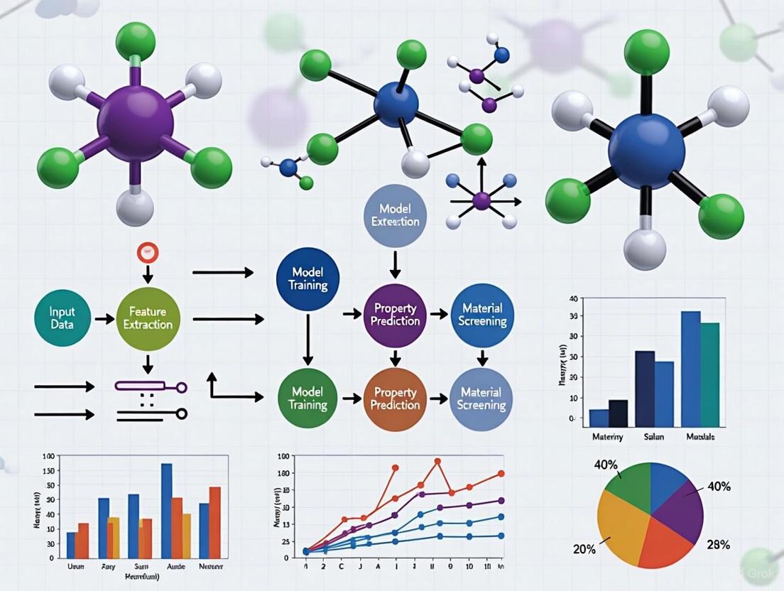
Visualizing the Workflow: From Data to Discovery

The following diagrams illustrate the logical flow of the AI-driven materials discovery process, from initial data handling to final validation.

Diagram 1: The AI-Driven Discovery Workflow.

Diagram 2: The ME-AI Framework for Explainable Discovery.

Successful implementation of data-driven materials discovery relies on a suite of computational and experimental tools. The following table catalogues key resources.

Table 2: Essential Research Reagent Solutions for AI-Driven Materials Discovery

Category	Item / Resource	Function and Application
Computational & Data Resources	Materials Project, OQMD, AFLOW, ICSD	Centralized databases providing crystal structures, thermodynamic properties, and band structures for model training [1].
	Graph Neural Networks (GNNs)	Deep learning models specifically designed to operate on graph-structured data, ideal for representing crystal structures and molecules [1].
	Bayesian Optimization (BO)	A sample-efficient optimization strategy for guiding experiments by balancing exploration and exploitation in complex parameter spaces [4].
	SHAP (SHapley Additive exPlanations)	An Explainable AI method that interprets the output of ML models, revealing the contribution of each input feature to a prediction [3].
Experimental & Robotic Systems	Liquid-Handling Robot	Automates the precise dispensing of precursor solutions for high-throughput synthesis of material libraries [4].
	Carbothermal Shock System	Enables rapid synthesis of nanomaterials (e.g., alloy catalysts) by quickly heating and cooling precursor materials [4].
	Automated Electrochemical Workstation	Performs high-throughput testing of functional properties, such as catalytic activity for fuel cells or battery performance [4].
	Automated Electron Microscope	Provides rapid microstructural and compositional analysis of synthesized materials without constant human operation [4].

The transition from trial-and-error to data-driven design is no longer a future prospect but a present reality in advanced materials research. Frameworks like ME-AI and platforms like CRESt exemplify how machine learning, explainable AI, and robotic automation are being integrated to create a powerful new paradigm for discovery. This approach not only accelerates the identification of novel materials with exceptional properties but also deepens fundamental scientific understanding by uncovering hidden structure-property relationships. As these tools become more sophisticated, accessible, and integrated with physical sciences, they promise to unlock a new era of innovation across energy, electronics, medicine, and beyond.

The field of materials science is undergoing a fundamental shift, moving from experience-driven and trial-and-error approaches to a data-driven research paradigm [7]. Machine learning (ML) has emerged as a transformative tool throughout the entire process of intelligent material innovation, enabling accelerated discovery, performance-optimized design, and efficient sustainable synthesis [8]. This paradigm change is largely driven by ML's ability to uncover intricate patterns within complex, high-dimensional materials data that are often challenging to identify through traditional methods [9].

ML techniques are revolutionizing materials research by providing powerful capabilities for predictive modeling and inverse design - where desired properties drive the discovery of new structures [10]. These approaches are significantly reducing the traditional 15-25 year timeline from material conception to deployment, hindering technological innovation across energy, healthcare, and electronics [7] [10]. The integration of computational methods with experimental validation has created new opportunities for tackling longstanding challenges in materials science, from improving corrosion resistance in magnesium alloys to developing novel catalyst materials for clean energy applications [4] [9].

This article provides a comprehensive overview of core ML techniques - supervised, unsupervised, and reinforcement learning - within the context of materials discovery and design. We present structured protocols, comparative analyses, and practical frameworks to equip researchers with the necessary tools to leverage these methodologies effectively in their materials research workflows.

Core Machine Learning Techniques in Materials Science

Machine learning encompasses various approaches that enable computers to learn from data and make decisions without explicit programming for every scenario [11]. In materials science, three primary paradigms have demonstrated significant utility: supervised learning, unsupervised learning, and reinforcement learning.

Supervised Learning

Supervised learning involves training algorithms on labeled datasets where each instance comprises an input object and a corresponding output value [7]. The fundamental characteristic of supervised learning is that the data are pre-categorized, including data classes, attributes, or specific feature locations [7]. After training on these labeled examples, the algorithm can map new, unseen inputs to appropriate outputs based on the learned patterns.

In materials science, supervised learning excels at property prediction and classification tasks, such as predicting mechanical properties based on composition or classifying crystal structures from diffraction data [7] [9]. These models establish correlations between material descriptors (composition, structure, processing parameters) and target properties (strength, conductivity, catalytic activity), enabling rapid screening of candidate materials without resource-intensive experiments or simulations [8].

Unsupervised Learning

Unsupervised learning operates on unlabeled data, seeking to identify inherent patterns, groupings, or structures without pre-defined categories [7]. These algorithms explore the data's natural organization, revealing hidden relationships that might not be apparent through manual analysis.

For materials research, unsupervised techniques are particularly valuable for materials categorization, pattern discovery in microstructure images, and dimensionality reduction of complex feature spaces [7]. By clustering materials with similar characteristics or reducing high-dimensional representations to more manageable forms, researchers can identify promising regions of materials space for further investigation and gain insights into fundamental structure-property relationships [10].

Reinforcement Learning

Reinforcement learning (RL) involves an agent learning to make decisions by interacting with an environment to maximize cumulative reward [7]. Through trial and error, the agent discovers optimal strategies or policies for achieving specific goals without requiring explicit examples of correct behavior.

In materials science, RL has found significant application in autonomous laboratories and synthesis optimization, where systems learn optimal processing parameters or synthesis routes through iterative experimentation [12] [4]. Algorithms such as proximal policy optimization (PPO) are increasingly important for controlling autonomous workflows, enabling systems to adaptively refine experimental conditions based on real-time feedback [12].

Table 1: Comparison of Core Machine Learning Techniques in Materials Research

Technique	Learning Paradigm	Primary Materials Applications	Key Advantages	Common Algorithms
Supervised Learning	Labeled training data	Property prediction, Classification, Quantitative structure-property relationship (QSPR) models	High accuracy for well-defined prediction tasks, Direct mapping from inputs to target properties	Artificial Neural Networks (ANNs), Support Vector Regression (SVR), Random Forests (RF), Gradient Boosting Machines (GBM)
Unsupervised Learning	Unlabeled data	Materials clustering, Dimensionality reduction, Pattern discovery in microstructures	Reveals hidden patterns without pre-existing labels, Reduces complexity of high-dimensional data	Principal Component Analysis (PCA), k-Means Clustering, Autoencoders, Generative Adversarial Networks (GANs)
Reinforcement Learning	Reward-based interaction with environment	Autonomous experimentation, Synthesis optimization, Processing parameter control	Adapts to complex, dynamic environments, Discovers novel strategies through exploration	Proximal Policy Optimization (PPO), Q-Learning, Deep Reinforcement Learning

Application Notes: ML Techniques in Materials Discovery

Supervised Learning for Property Prediction

Supervised learning has become indispensable for predicting material properties across diverse systems, from magnesium alloys to catalytic materials. The ability to establish accurate relationships between material characteristics and performance metrics has significantly reduced reliance on costly experimental characterization and computational simulations [9].

In practice, supervised models have demonstrated remarkable success in predicting mechanical properties such as yield strength, tensile strength, and fatigue life based on composition and processing parameters [9]. For magnesium alloys, models including Artificial Neural Networks (ANNs), Support Vector Regression (SVR), and Random Forests (RF) have achieved accurate predictions of mechanical behavior under various thermomechanical processing conditions [9]. Similarly, in catalyst development, supervised learning can correlate elemental composition and coordination environments with catalytic activity and resistance to poisoning species [4].

The effectiveness of supervised learning extends to microstructural analysis, where Convolutional Neural Networks (CNNs) can extract features from micrograph images to predict material properties or classify structural characteristics [9]. These image-based approaches enable rapid assessment of microstructure-property relationships that traditionally required meticulous manual analysis.

Unsupervised Learning for Materials Exploration

Unsupervised learning techniques empower researchers to navigate complex materials spaces without pre-existing labels or categories. By allowing the data to reveal its inherent structure, these methods facilitate novel materials discovery and hypothesis generation.

A prominent application involves using clustering algorithms to identify groups of materials with similar characteristics, enabling researchers to discover new material families or identify outliers with unusual properties [10]. In catalytic materials research, unsupervised learning has helped categorize catalyst compositions based on performance descriptors, guiding the exploration of promising compositional spaces [8].

Dimensionality reduction techniques such as Principal Component Analysis (PCA) and autoencoders transform high-dimensional materials representations (such as crystal structure descriptors or compositional features) into lower-dimensional spaces while preserving essential information [4]. This transformation facilitates visualization of materials relationships and identification of fundamental design principles that govern material behavior [10].

Reinforcement Learning for Autonomous Experimentation

Reinforcement learning represents a paradigm shift in experimental materials science, enabling autonomous systems that learn optimal strategies through direct interaction with laboratory environments. These approaches are particularly valuable for problems where the relationship between processing parameters and material outcomes is complex and not fully understood.

In autonomous laboratories, RL agents control robotic systems for materials synthesis and characterization, continuously refining their strategies based on experimental outcomes [12] [4]. For example, systems can learn optimal synthesis recipes for multielement catalysts by adjusting precursor ratios, processing temperatures, and reaction times to maximize target properties such as catalytic activity or stability [4].

RL also excels at adaptive experimental design, where systems dynamically adjust their exploration strategy based on accumulating results. This capability is particularly valuable for resource-intensive experiments, as it focuses resources on promising regions of parameter space [12]. By balancing exploration of unknown regions with exploitation of known promising areas, RL systems can efficiently navigate complex optimization landscapes.

Table 2: Representative Applications of ML Techniques in Materials Science

Material Category	Supervised Learning Application	Unsupervised Learning Application	Reinforcement Learning Application
Magnesium Alloys	Predicting yield strength and corrosion behavior from composition and processing parameters [9]	Clustering alloy compositions with similar deformation mechanisms [9]	Optimizing thermomechanical processing parameters [9]
Catalytic Materials	Predicting catalytic activity from elemental composition and coordination environment [4]	Identifying descriptor relationships for catalytic performance [8]	Autonomous optimization of multielement catalyst synthesis [4]
Energy Materials	Forecasting battery cycle life from early-cycle data [7]	Categorizing crystal structures for ion conduction [10]	Self-driving labs for photovoltaic material discovery [2]
Polymeric Materials	Relating monomer composition to mechanical properties [8]	Mapping the chemical space of biodegradable polymers [10]	Optimizing polymerization reaction conditions [12]

Experimental Protocols

Protocol: Supervised Learning for Mechanical Property Prediction

This protocol outlines the workflow for developing supervised learning models to predict mechanical properties of materials based on composition and processing parameters, with specific application to magnesium alloys [9].

Data Collection and Preprocessing

• Data Acquisition: Compile a comprehensive dataset from experimental measurements, computational simulations, or literature sources. Essential features include alloy composition (elemental percentages), processing parameters (extrusion temperature, speed, heat treatment conditions), and target mechanical properties (yield strength, ultimate tensile strength, elongation) [9].
• Data Cleaning: Address missing values through appropriate imputation methods or removal of incomplete records. Identify and handle outliers that may result from measurement errors using statistical methods (e.g., Z-score analysis) [9].
• Feature Engineering: Create domain-informed descriptors such as atomic size mismatch, electronegativity differences, and processing-derived parameters (Zener-Hollomon parameter for thermomechanical processing) [9].
• Data Normalization: Apply standardization (scaling to zero mean and unit variance) or min-max scaling to ensure all features contribute equally to model training [7].

Model Training and Validation

• Dataset Partitioning: Split data into training (70-80%), validation (10-15%), and test sets (10-15%) using stratified sampling to maintain distribution of target variables across splits [9].
• Algorithm Selection: Implement multiple algorithms including Artificial Neural Networks (ANNs), Support Vector Regression (SVR), and Random Forests (RF) to compare performance [9].
• Hyperparameter Tuning: Optimize model-specific parameters through grid search or Bayesian optimization, using cross-validation on the training set to prevent overfitting [9].
• Model Validation: Evaluate performance on the held-out test set using metrics relevant to regression tasks: Mean Absolute Error (MAE), Root Mean Square Error (RMSE), and Coefficient of Determination (R²) [9].

Model Interpretation and Deployment

• Feature Importance Analysis: Employ permutation importance, SHAP values, or model-specific importance measures to identify dominant factors controlling mechanical properties [9].
• Domain Knowledge Integration: Validate model insights against established metallurgical principles to ensure physical plausibility [9].
• Deployment for Prediction: Utilize the trained model to screen proposed alloy compositions and processing parameters, prioritizing promising candidates for experimental verification [9].

Protocol: Reinforcement Learning for Autonomous Materials Synthesis

This protocol details the implementation of reinforcement learning for autonomous optimization of synthesis parameters, with specific application to multielement catalyst discovery [4].

Environment Setup

• State Representation: Define the state space encompassing controllable synthesis parameters (precursor concentrations, temperature, pressure, reaction time) and characterization data (in-situ spectroscopy, microscopy) when available [4].
• Action Space Definition: Establish discrete or continuous actions corresponding to adjustments of synthesis parameters within experimentally feasible ranges [4].
• Reward Function Design: Formulate a reward function based on target material properties (catalytic activity, selectivity, stability) measured through high-throughput characterization [4].

Agent Training

• Algorithm Selection: Implement Deep Reinforcement Learning algorithms such as Proximal Policy Optimization (PPO) or Deep Q-Networks (DQN) capable of handling high-dimensional state and action spaces [12] [4].
• Exploration Strategy: Balance exploration and exploitation using approaches such as ε-greedy or adding noise to parameter space, ensuring adequate coverage of the synthesis space [4].
• Experience Replay: Store state-action-reward transitions in a replay buffer and sample batches for training to improve data efficiency and stabilize learning [4].
• Training Iteration: Cycle through action selection, environment interaction, reward computation, and policy updates until performance converges or reaches target thresholds [4].

Experimental Validation

• Robotic Integration: Deploy the trained policy on robotic synthesis platforms capable of executing specified synthesis protocols with minimal human intervention [4].
• Closed-Loop Operation: Implement real-time characterization and feedback to continuously update the policy based on experimental outcomes [4].
• Human Oversight: Maintain researcher supervision for safety-critical decisions and validation of novel discoveries [4].

Diagram 1: RL for autonomous synthesis workflow

The Scientist's Toolkit: Research Reagent Solutions

Successful implementation of ML-driven materials research requires both computational tools and experimental resources. The following table outlines essential components for establishing an integrated computational-experimental workflow.

Table 3: Essential Research Reagents and Tools for ML-Driven Materials Research

Category	Item	Specification/Function	Application Examples
Computational Framework	Core ML Framework	Convert trained models from popular deep learning frameworks (Caffe, Keras, SKLearn) for device deployment [11]	iOS app integration for on-device predictions [11]
Data Management	FAIR Data Infrastructure	Ensure Findability, Accessibility, Interoperability, and Reusability of materials data [12]	Standardized data sharing across research institutions [12]
Automation Equipment	Liquid-Handling Robot	Precise dispensing of precursor solutions for high-throughput synthesis [4]	Multielement catalyst library preparation [4]
Characterization Tools	Automated Electrochemical Workstation	High-throughput measurement of catalytic activity and stability [4]	Fuel cell catalyst performance evaluation [4]
Structural Analysis	Automated Electron Microscopy	Microstructural characterization with minimal human intervention [4]	Grain size distribution analysis in alloys [9]
Synthesis Systems	Carbothermal Shock System	Rapid synthesis of materials through extreme temperature jumps [4]	Nanomaterial and catalyst preparation [4]
Experimental Monitoring	Computer Vision System	Visual monitoring of experiments for reproducibility assessment [4]	Detection of deviations in sample morphology or placement [4]
Neodidymelliosides A	Neodidymelliosides A, MF:C51H96O13, MW:917.3 g/mol	Chemical Reagent	Bench Chemicals
SARS-CoV-2-IN-73	SARS-CoV-2-IN-73, MF:C17H18FN3O8, MW:411.3 g/mol	Chemical Reagent	Bench Chemicals

Integrated Workflow for ML-Driven Materials Discovery

The full potential of machine learning in materials science emerges when multiple techniques are integrated into a cohesive discovery pipeline. This integrated approach combines computational predictions with experimental validation in a closed-loop system that continuously refines models based on new data.

Diagram 2: Integrated ML-driven discovery workflow

The workflow begins with clearly defined target properties, which guide generative models in proposing candidate materials with desired characteristics [10]. These candidates undergo computational screening through supervised learning models that predict key properties, followed by unsupervised clustering to identify promising material families and diverse candidates [10] [9]. Reinforcement learning then guides autonomous synthesis systems in producing selected candidates, with high-throughput characterization providing experimental validation [4]. Results feed back into the ML models, creating a continuous improvement cycle that refines predictions with each iteration [4].

This integrated approach has demonstrated remarkable success in various materials discovery campaigns. For example, in fuel cell catalyst development, such workflows have explored over 900 chemistries and conducted 3,500 electrochemical tests, leading to the discovery of multielement catalysts with record power density despite containing only one-fourth the precious metals of previous designs [4]. Similarly, in magnesium alloy research, combined ML and experimental approaches have accelerated the design of alloys with improved corrosion resistance and mechanical properties [9].

The future of ML-driven materials discovery lies in enhancing these integrated workflows through improved data standards, physics-informed model architectures, and more sophisticated autonomous laboratories. As these technologies mature, they will increasingly enable researchers to navigate the vast complexity of materials space efficiently, accelerating the development of advanced materials to address critical challenges in energy, sustainability, and healthcare.

Navigating the Vast Chemical Space with Unsupervised Learning and Dimensionality Reduction

The exploration of chemical space, encompassing all possible organic and inorganic molecules, is a fundamental challenge in materials science and drug discovery. With chemical libraries containing millions of compounds, researchers face significant cognitive and computational barriers in analyzing this wealth of data. This application note details how unsupervised learning and dimensionality reduction methods are enabling scientists to visualize, navigate, and extract meaningful patterns from these vast chemical datasets. We provide experimental protocols for implementing these techniques, supported by case studies and quantitative comparisons of their performance in real-world materials discovery applications. Framed within the broader context of machine learning-driven materials research, these methodologies are proving essential for identifying novel functional materials and bioactive compounds beyond the boundaries of previously charted chemical regions.

The "Big Data" era in medicinal chemistry and materials science presents new challenges for analysis, as modern computers can store and process millions of molecular structures, yet final decisions remain in human hands [13]. The ability of humans to analyze large chemical data sets is limited by cognitive constraints, creating a critical demand for methods and tools to visualize and navigate chemical space [13]. The chemical space of possible materials is astronomically large, with recent expansions through computational methods identifying 2.2 million stable crystal structures—an order-of-magnitude increase from previously known materials [14].

Within this context, unsupervised learning and dimensionality reduction techniques have emerged as essential tools for making sense of this complexity. These approaches allow researchers to project high-dimensional molecular descriptors into lower-dimensional representations that can be visually inspected and analyzed. This capability is particularly valuable for identifying clusters of compounds with similar properties, detecting outliers, and generating hypotheses for further exploration. As the field advances, these methods are evolving to address increasingly large and complex datasets, enabling the discovery of structurally novel molecules with desired properties [15] [13].

Computational Foundations

The Chemical Space Navigation Problem

Chemical space is fundamentally high-dimensional, with each potential molecule represented by hundreds of descriptors capturing structural, electronic, and physicochemical properties. The core challenge in navigating this space lies in the sheer combinatorial complexity of possible molecular structures. Recent advances have demonstrated that graph networks trained at scale can reach unprecedented levels of generalization, improving the efficiency of materials discovery by an order of magnitude [14]. This approach has led to the discovery of 2.2 million structures below the convex hull, many of which escaped previous human chemical intuition [14].

Key Algorithms and Approaches

Table 1: Dimensionality Reduction Methods for Chemical Space Analysis

Method	Key Principles	Advantages in Chemical Context	Limitations
PCA (Principal Component Analysis)	Linear projection that maximizes variance	Computational efficiency, interpretability of components	Limited capacity for nonlinear relationships
t-SNE (t-Distributed Stochastic Neighbor Embedding)	Preserves local neighborhoods in high-dim space	Effective cluster visualization, preserves local structure	Computational intensity, global structure loss
UMAP (Uniform Manifold Approximation and Projection)	Preserves topological structure of data	Faster than t-SNE, better global structure preservation	Parameter sensitivity, theoretical complexity
Autoencoders	Neural network learns compressed representation	Handles nonlinearity, can generate new structures	Training complexity, data requirements
Generative Topographic Mapping (GTM)	Probabilistic alternative to SOM	Probabilistic framework, principled initialization	Computational demand for large datasets

The selection of appropriate dimensionality reduction techniques depends on the specific objectives of the chemical space analysis. For initial exploration and visualization, UMAP has gained popularity due to its speed and ability to preserve both local and global structure [13]. For generative purposes, deep learning approaches such as autoencoders provide powerful frameworks for both compression and molecular generation [15] [14].

Recent advances have extended chemical space visualization beyond chemical compounds to include reactions and chemical libraries [13]. Deep generative modeling combined with chemical space visualization is paving the way for interactive exploration of chemical space, enabling researchers to navigate efficiently through regions of interest and identify promising candidates for synthesis and testing.

Experimental Protocols

Protocol 1: Chemical Space Mapping with UMAP

Purpose: To create a two-dimensional visualization of a high-dimensional chemical library for cluster identification and novelty assessment.

Materials and Reagents:

• Chemical dataset (e.g., ChEMBL, ZINC, Materials Project)
• Molecular descriptors (e.g., ECFP fingerprints, Mordred descriptors)
• Python environment with umap-learn, RDKit, pandas, numpy
• Computational resources (minimum 8GB RAM for datasets <100,000 compounds)

Procedure:

• Data Preparation:
  • Load molecular structures from SDF or SMILES format
  • Compute molecular descriptors or fingerprints

• Dimensionality Reduction:

  • Initialize UMAP with optimized parameters for chemical space

  • Fit transform the descriptor matrix

• Visualization and Cluster Analysis:

  • Create scatter plots colored by property values
  • Identify clusters using HDBSCAN or DBSCAN
  • Annotate clusters with molecular properties

• Novelty Assessment:

  • Calculate "unfamiliarity" metric based on reconstruction error [15]
  • Identify regions of chemical space distant from training data

Troubleshooting:

• For large datasets (>1M compounds), consider using PCA initialization
• Adjust n_neighbors parameter to balance local and global structure
• For heterogeneous datasets, try different distance metrics (Euclidean, Jaccard, Cosine)

Protocol 2: Molecular Reconstruction for Generalizability Assessment

Purpose: To estimate model generalizability and identify out-of-distribution molecules using joint modeling of molecular property prediction with molecular reconstruction.

Materials and Reagents:

• Pre-trained molecular autoencoder
• Bioactivity dataset with known measurements
• Python with deep learning framework (PyTorch/TensorFlow)
• GPU acceleration recommended

Procedure:

• Model Architecture Setup:
  • Implement joint architecture with property prediction and reconstruction heads
  • Use graph neural networks or sequence-based encoders
  • Share encoder weights between both tasks

• Training Protocol:

  • Split data into training and validation sets using time-split or scaffold-split

  • Train with multi-task loss function:

• Unfamiliarity Metric Calculation:

  • Compute reconstruction error for new molecules
  • Normalize error relative to training set distribution
  • Set thresholds for familiarity classification

• Validation:

  • Test on known bioactivity datasets (e.g., kinase inhibitors)
  • Correlate unfamiliarity with prediction accuracy drop
  • Experimental validation of unfamiliar compounds [15]

Validation Results: This approach has been experimentally validated for two clinically relevant kinases, discovering seven compounds with low micromolar potency and limited similarity to training molecules [15].

Visualization Workflows

The following diagram illustrates the integrated workflow for chemical space navigation combining dimensionality reduction with generalizability assessment:

Chemical Space Navigation Workflow

Research Reagents and Computational Tools

Table 2: Essential Research Reagents and Computational Tools for Chemical Space Exploration

Tool/Resource	Type	Function	Application Example
RDKit	Open-source cheminformatics toolkit	Molecular descriptor calculation, fingerprint generation	ECFP generation for similarity analysis
UMAP	Dimensionality reduction library	Non-linear dimensionality reduction	2D visualization of compound libraries
GNoME	Graph neural network model	Materials stability prediction	Discovery of novel crystal structures [14]
Materials Project	Database	Crystallographic and computational data	Training data for materials discovery models
ChEMBL	Database	Bioactivity data for drug-like molecules	Mapping bioactivity landscapes
Autoencoders	Neural network architecture	Learning compressed molecular representations	Molecular generation and novelty detection [15]
AlphaFold	Protein structure prediction	Predicting protein 3D structures	Target-informed chemical space navigation [16]

Applications in Materials Discovery and Drug Development

Case Study: Scaling Deep Learning for Materials Discovery

The Graph Networks for Materials Exploration (GNoME) project exemplifies the power of combining advanced machine learning with chemical space navigation. Through large-scale active learning, GNoME models have discovered 2.2 million crystal structures stable with respect to previous work, with 381,000 new entries on the updated convex hull [14]. This represents an order-of-magnitude expansion from all previous discoveries.

Key to this success was the development of models that generalize effectively beyond their training data. The GNoME approach demonstrated emergent out-of-distribution generalization, accurately predicting structures with five or more unique elements despite their omission from initial training [14]. This capability provides one of the first efficient strategies to explore this combinatorially large region of chemical space.

Table 3: Performance Metrics for GNoME Materials Discovery [14]

Metric	Initial Performance	Final Performance	Improvement Factor
Stability Prediction Hit Rate	<6%	>80%	>13x
Energy Prediction Error	21 meV/atom	11 meV/atom	1.9x
Stable Materials Discovered	48,000 (baseline)	421,000	8.8x
Novel Prototypes Identified	8,000 (baseline)	45,500	5.6x

Case Study: AI-Driven Drug Discovery

In pharmaceutical applications, chemical space navigation enables more efficient exploration of potential drug candidates. AI technologies play an essential role in molecular modeling, drug design and screening, with demonstrated capabilities to lower costs and shorten development timelines [16]. For instance, Insilico Medicine developed an AI-driven drug discovery system that designed a novel drug candidate for idiopathic pulmonary fibrosis in just 18 months, significantly faster than traditional approaches [16].

The "unfamiliarity" metric introduced through joint modeling approaches addresses a critical challenge in molecular machine learning: the inability of models to generalize beyond the chemical space of their training data [15]. By combining molecular property prediction with molecular reconstruction, this approach provides a quantitative measure to estimate model generalizability and identify promising compounds that are structurally novel yet likely to maintain desired properties.

Concluding Remarks

The navigation of chemical space through unsupervised learning and dimensionality reduction has transformed from a niche analytical technique to an essential component of modern materials discovery and drug development pipelines. As chemical libraries continue to grow—with projects like GNoME adding millions of new stable structures—these methods will become increasingly critical for identifying promising candidates for synthesis and testing [14].

Future directions in this field point toward more sustainable and efficient exploration of chemical spaces. Recent initiatives like the SusML workshop focus on developing Efficient, Accurate, Scalable, and Transferable (EAST) methodologies that minimize energy consumption and data storage while creating robust ML models [17] [18]. Similarly, the integration of human expertise through human-in-the-loop approaches and large language models shows promise for improving out-of-domain performance with reduced data requirements [19].

The ongoing challenge of navigating chemical space reflects the broader objectives of materials discovery and design using machine learning: to expand beyond the boundaries of human chemical intuition while providing interpretable, actionable insights that accelerate the discovery of novel functional materials and therapeutic agents.

Foundation models, characterized by their training on broad data using self-supervision at scale and their adaptability to a wide range of downstream tasks, represent a paradigm shift in artificial intelligence applications for materials science [20]. These models, built upon transformer architectures, decouple the data-hungry task of representation learning from specific downstream applications, enabling powerful predictive and generative capabilities even with limited labeled data [20]. Within materials informatics, this approach is accelerating the discovery and design of novel materials with tailored properties, offering solutions to long-standing challenges in sustainability, energy storage, and semiconductor technology [21].

Current State of Foundation Models in Materials Discovery

Architectural Foundations and Modalities

Foundation models for materials discovery employ diverse architectural strategies and molecular representations, each with distinct advantages and limitations. Encoder-only models, derived from the BERT architecture, excel at understanding and representing input data for property prediction tasks, while decoder-only models are optimized for generating new chemical entities [20]. The representation of molecular structures presents a fundamental challenge, with current approaches utilizing multiple modalities:

• Text-based Representations: SMILES (Simplified Molecular-Input Line-Entry System) and SELFIES (Self-Referencing Embedded Strings) convert molecular structures into text strings, enabling the application of natural language processing techniques [21]. While SMILES databases contain approximately 1.1 billion molecules, this representation can lose valuable 3D structural information and sometimes generates invalid molecules [21].
• Graph-based Representations: Molecular graphs capture the spatial arrangement of atoms and their bonds, preserving structural information at the cost of higher computational requirements [21].
• Experimental Data Modalities: Spectrograms and other experimental measurements provide empirical data on molecular behavior but may be incomplete or contain errors [21].

Table 1: Comparison of Molecular Representation Modalities in Foundation Models

Representation Type	Example	Advantages	Limitations	Training Data Scale
Text-based	SMILES, SELFIES	Leverages NLP techniques; large datasets available	Loses 3D structural information; may generate invalid molecules	~1.1 billion molecules (SMILES) [21]
Graph-based	Molecular Hypergraphs	Captures spatial atom arrangements	Computationally intensive	~1.4 million graphs [21]
3D Structural	Crystal Graph Representations	Preserves spatial relationships	Limited dataset availability	Smaller than 2D representations [20]
Multimodal	Mixture of Experts	Combines strengths of multiple representations	Increased complexity	Varies by component models

Data Extraction and Curation

The development of effective foundation models requires significant volumes of high-quality materials data, presenting substantial extraction and curation challenges. Chemical databases such as PubChem, ZINC, and ChEMBL provide structured information but are often limited by licensing restrictions, dataset size, and biased data sourcing [20]. Modern data extraction approaches must parse information from multiple modalities within scientific documents, including text, tables, images, and molecular structures [20].

Advanced extraction methodologies include:

• Named Entity Recognition (NER): Identifies materials and compounds within text passages [20]
• Computer Vision Approaches: Vision Transformers and Graph Neural Networks extract molecular structures from images in documents [20]
• Specialized Algorithms: Tools like Plot2Spectra extract data points from spectroscopy plots, while DePlot converts visual representations into structured tabular data [20]
• Schema-based Extraction: Leverages recent advances in large language models for accurate property extraction and association [20]

Application Notes: Key Use Cases and Performance

Property Prediction

Foundation models demonstrate remarkable capabilities in predicting material properties from structure, enabling rapid screening of candidate materials. Current models predominantly utilize 2D representations (SMILES, SELFIES), though this approach omits potentially critical 3D conformational information [20]. An exception exists for inorganic solids like crystals, where property prediction models typically leverage 3D structures through graph-based or primitive cell feature representations [20].

The IBM FM4M project has demonstrated that multi-modal approaches significantly enhance prediction accuracy. Their Mixture of Experts (MoE) architecture, which combines SMILES, SELFIES, and molecular graph representations, outperformed single-modality models on the MoleculeNet benchmark, achieving superior performance on both classification tasks (e.g., predicting toxicity) and regression tasks (e.g., predicting water solubility) [21].

Table 2: Property Prediction Performance of Foundation Models on MoleculeNet Benchmarks

Model Architecture	Representation Modality	Classification Accuracy	Regression Performance	Notable Applications
Encoder-only (BERT-like)	SMILES/SELFIES	High for electronic properties	Moderate for quantum properties	Topological material identification [20] [6]
Decoder-only (GPT-like)	SMILES/SELFIES	Moderate	High for synthetic accessibility	Molecular generation [20]
Graph Neural Networks	Molecular Graphs	High for mechanically-relevant properties	High for formation energies	Crystal property prediction [20]
Multi-modal MoE	Combined embeddings	Highest overall	Highest overall	Broad applicability across tasks [21]

Molecular Generation and Inverse Design

Beyond property prediction, foundation models enable inverse design—generating novel molecular structures with desired properties. Decoder-only architectures are particularly suited to this task, sequentially generating molecular representations token-by-token [20]. These models can be conditioned to explore specific regions of the property distribution through alignment processes, ensuring generated structures exhibit desired characteristics such as improved synthesizability or chemical correctness [20].

Expert-Informed Discovery

The ME-AI (Materials Expert-Artificial Intelligence) framework demonstrates how expert intuition can be translated into quantitative descriptors through foundation models. In one implementation, researchers trained a Gaussian-process model on 879 square-net compounds using 12 experimental features, combining electronic structure information (electron affinity, electronegativity, valence electron count) with structural parameters [6]. The model not only recovered the known structural "tolerance factor" descriptor but also identified hypervalency as a decisive chemical factor in identifying topological semimetals [6]. Remarkably, the model demonstrated transferability, correctly classifying topological insulators in rocksalt structures despite being trained only on square-net topological semimetal data [6].

Experimental Protocols

Protocol: Multi-modal Foundation Model Training

Purpose: To train a foundation model that leverages multiple molecular representations for enhanced materials property prediction.

Materials and Methods:

• Data Collection:
  • Gather SMILES representations from PubChem and ZINC-22 databases (≈1 billion validated samples) [21]
  • Collect molecular graph data with atomic number and charge information (≈1.4 million graphs) [21]
  • Curate experimental data from literature and databases, ensuring quality control

• Pre-training:

  • Train SMILES-TED (Transformer Encoder-Decoder) on 91 million SMILES samples [21]
  • Train SELFIES-TED on 1 billion SELFIES samples [21]
  • Train MHG-GED (Molecular Hypergraph Grammar) on graph representations [21]
  • Utilize self-supervised learning objectives appropriate for each modality

• Multi-modal Fusion:

  • Implement Mixture of Experts (MoE) architecture with router algorithm
  • Train router to selectively activate modality-specific "experts" based on task requirements
  • Fine-tune on downstream tasks using labeled datasets

• Validation:

  • Evaluate on MoleculeNet benchmark tasks
  • Compare performance against single-modality baselines
  • Analyze expert activation patterns to understand modality contributions [21]

Protocol: Automated Materials Discovery with CRESt Platform

Purpose: To implement a closed-loop materials discovery system integrating foundation models with robotic experimentation.

Materials and Methods:

• System Setup:
  • Deploy liquid-handling robot for sample preparation
  • Integrate carbothermal shock system for rapid material synthesis
  • Set up automated electrochemical workstation for testing
  • Install characterization equipment (automated electron microscopy, optical microscopy)
  • Configure computer vision system with cameras for experiment monitoring [4]

• Workflow Implementation:

  • Natural language interface for researcher instructions
  • Knowledge embedding from scientific literature using foundation models
  • Principal component analysis in knowledge embedding space to reduce search dimensionality
  • Bayesian optimization in reduced space for experiment design [4]

• Active Learning Cycle:

  • Robotically synthesize materials based on model recommendations
  • Automatically characterize structure and test performance
  • Feed experimental results back into foundation models
  • Incorporate human feedback via natural language [4]

• Validation:

  • Track reproducibility across experimental iterations
  • Monitor system-identified issues and suggested corrections
  • Evaluate final material performance against project objectives

Visualization Diagrams

Foundation Model Architecture for Materials Informatics

CRESt Automated Discovery Workflow

The Scientist's Toolkit: Essential Research Reagents

Table 3: Essential Research Reagents and Computational Resources for Foundation Model Applications

Resource Category	Specific Examples	Function/Application	Key Characteristics
Chemical Databases	PubChem, ZINC, ChEMBL, ICSD	Training data for foundation models; reference for validation	Large-scale structured information; variable quality and completeness [20]
Representation Libraries	RDKit, SMILES, SELFIES	Molecular representation and conversion	Standardized formats; enable NLP approaches to chemistry [21]
Pre-trained Models	SMILES-TED, SELFIES-TED, MHG-GED	Transfer learning for specific materials tasks	Reduced data requirements; improved performance on specialized tasks [21]
Benchmark Datasets	MoleculeNet, Materials Project	Model evaluation and comparison	Standardized tasks; enable performance comparisons [21]
Automation Equipment	Liquid-handling robots, Automated electrochemical workstations	High-throughput experimentation	Enable rapid experimental validation; reduce human error [4]
Characterization Tools	Automated electron microscopy, X-ray diffraction	Structural analysis of synthesized materials	Provide ground truth data for model validation [4]
Krasg12D-IN-2	Krasg12D-IN-2, MF:C34H31F4N7O, MW:631.7 g/mol	Chemical Reagent	Bench Chemicals
Asct2-IN-2	Asct2-IN-2, MF:C44H50N2O4, MW:670.9 g/mol	Chemical Reagent	Bench Chemicals

Foundation models represent a transformative approach to materials informatics, leveraging pre-trained transformers to accelerate property prediction, molecular generation, and experimental design. The integration of multiple molecular representations through architectures like Mixture of Experts demonstrates enhanced performance across diverse tasks, while platforms such as CRESt showcase the potential for closed-loop discovery systems combining AI with robotic experimentation. As these models continue to evolve, they promise to significantly reduce the time and cost associated with materials development, addressing critical challenges in sustainability, energy, and electronics.

The integration of public materials databases and machine learning (ML) is revolutionizing the field of materials science, creating a new paradigm for accelerated materials discovery and design. Foundational databases like the Materials Project and AFLOW provide vast, pre-computed datasets of material properties, serving as the essential fuel for data-driven research. These resources provide the high-quality, consistently calculated data required to train, benchmark, and validate ML models, enabling the prediction of novel materials and properties with unprecedented speed. This application note details the methodologies for effectively leveraging these databases within an ML-driven research workflow, providing protocols for data access, featurization, and model benchmarking to empower researchers in pushing the frontiers of materials informatics.

The Materials Project and AFLOW represent two pillars of the materials genomics initiative, both offering immense volumes of data but with distinct emphases and integrated tooling. The table below provides a quantitative comparison of their core offerings.

Table 1: Core Features of Public Materials Databases

Feature	Materials Project (MP)	AFLOW++ Framework
Primary Goal	Accelerate materials design by computing properties of inorganic crystals and molecules [22].	Autonomous materials design via an interconnected collection of algorithms and workflows [23].
Data Scope	Pre-computed properties for materials and molecules; includes data from other sources in MatBench [24].	High-throughput calculation of structural, electronic, thermodynamic, and thermomechanical properties [23].
Sample Datasets	MatBench curates datasets from 312 to 132,000 entries; includes both experimental and calculated data [24].	Heavily used for disordered systems, high-entropy ceramics, and bulk metallic glasses [23].
Key Properties	Electronic, thermal, thermodynamic, and mechanical properties [24].	Stability/synthesizability, electronic structure, elastic constants, and thermomechanical properties [23].
Unique Tools	MatBench benchmarking suite; integration with Matminer for featurization [24].	PAOFLOW (electronic analysis), AEL/AGL (elasticity/Gibbs), modules for disorder (POCC, QCA) [23].
Interoperability	Data accessible via API, Python package, and direct download [24].	Prioritizes interoperability and consistency; integrated with VASP, Quantum ESPRESSO, and others [23].

Experimental Protocols for ML-Driven Materials Research

Protocol 1: Bulk Data Acquisition via OPTIMADE API

Acquiring large, clean datasets is the critical first step in any ML pipeline. The OPTIMADE API provides a standardized interface for querying multiple materials databases, including AFLOW.

Application: Benchmarking a Bayesian Optimization framework for crystal structures [25].

Research Reagent Solutions:

• OPTIMADE Client (optimade Python package): A community-standard API for accessing materials data across different providers.
• ASE (Atomic Simulation Environment): A Python package for working with atoms and structures; used for file format conversion.
• AFLOW Provider: One of the primary OPTIMADE providers, offering access to the AFLOW database's calculated properties.

Methodology:

• Client Initialization: Initialize the OptimadeClient and target the AFLOW provider to restrict the data source.

• Query Filtering: Apply a filter to select records with specific known properties, such as heat capacity at 300K.

• Pagination Handling: The client's get method handles pagination automatically. Extract the structure data from the result object.

• Data Conversion and Storage: Iterate through the returned structures, convert them to a standard format (e.g., CIF) using an adapter, and save them to disk alongside a CSV file logging the target property.

Note: Be mindful of potential download limits (e.g., 1,000 records per query) [25]. For larger datasets, implement looping with pagination tokens or use provider-specific bulk download options where available.

Protocol 2: End-to-End ML Model Benchmarking with MatBench

MatBench provides a standardized framework for evaluating and comparing the performance of ML models on various materials property prediction tasks, similar to the role of ImageNet in computer vision [24].

Application: Objectively evaluating a new graph neural network model for predicting material band gaps.

Research Reagent Solutions:

• MatBench Python package: Provides easy access to curated benchmark datasets.
• Matminer: A Python toolbox for data featurization and mining, often used in conjunction with MatBench.
• Automatminer: An "AutoML" pipeline that automates featurization, model selection, and hyperparameter tuning.

Methodology:

• Dataset Selection: Load a specific benchmark task from MatBench. For band gap prediction, the MatBench_mp_gap dataset is appropriate.

• Model Definition: Define your custom ML model (e.g., a PyTorch or scikit-learn model). The model must adhere to the scikit-learn estimator API.

• Benchmark Execution: Run the benchmark, which automatically handles data splitting into training and test sets.

• Performance Analysis and Submission: Use MatBench's built-in functions to analyze model performance across all folds and datasets. The results can be formally submitted to the public MatBench leaderboard for comparison with state-of-the-art models [24].

The following workflow diagram illustrates the iterative process of model benchmarking and improvement.

Community Benchmarks and Emerging Frontiers

The field is rapidly evolving with the establishment of robust benchmarks and a focus on next-generation challenges. The table below summarizes key benchmarking and community initiatives.

Table 2: Key Benchmarks and Community Initiatives in AI for Materials

Initiative	Primary Focus	Role in ML Research
MatBench [24]	Materials property prediction.	Provides a suite of curated datasets for training and a public leaderboard for objective model comparison, defining state-of-the-art.
MLIP Arena [26]	Machine Learning Interatomic Potentials.	An open benchmark platform for ensuring fairness and transparency in evaluating interatomic potentials.
AI4Mat Workshop Series (ICLR & NeurIPS 2025) [26] [27]	Foundation models, representations, and benchmarking.	A leading venue for discussing limitations of current benchmarks and fostering development of methods with real-world impact.

A central theme in current research is moving beyond traditional benchmarks to address core technical challenges. As highlighted in recent workshops, the community is focused on two key questions:

• How Do We Build a Foundation Model for Materials Science? There is growing interest in developing large-scale, pre-trained models that can be adapted to a wide range of downstream materials tasks [26].
• What are Next-Generation Representations of Materials Data? Research continues into creating more powerful and data-efficient representations of crystal structures, molecules, and their multi-modal data (e.g., text, images) [26].

Essential Software Toolkit

A robust software ecosystem has emerged to support every stage of the ML research workflow, from data access to model deployment.

Table 3: Essential Software Tools for ML-Based Materials Discovery

Tool	Language	Primary Function	Application Example
AFLOW++ [23]	C++/Python	High-throughput generation and calculation of materials properties.	Automating the input generation and calculation of elastic constants for a new class of high-entropy carbides.
Matminer [24]	Python	Featurization of materials primitives (crystals, molecules) and dataset creation.	Converting a set of CIF files into a feature matrix of composition and structural descriptors for model training.
Automatminer [24]	Python	Automated machine learning (AutoML) pipeline for materials property prediction.	Rapidly prototyping and deploying a predictive model for bulk modulus with minimal human intervention.
PAOFLOW [23]	Python	Post-processing of electronic structures to compute advanced properties (e.g., transport, topological).	Calculating the anomalous Hall conductivity from a set of first-principles calculation results.
Antiviral agent 45	Antiviral agent 45, MF:C47H94N6O6P2, MW:901.2 g/mol	Chemical Reagent	Bench Chemicals
Antimalarial agent 27	Antimalarial agent 27, MF:C10H11NNaO5P, MW:279.16 g/mol	Chemical Reagent	Bench Chemicals

The logical relationship and data flow between these core tools, databases, and the researcher are visualized below.

From Prediction to Creation: ML Methodologies for Property Prediction and Generative Design

The discovery and development of new functional materials are pivotal for technological progress, from renewable energy systems to advanced electronics and pharmaceuticals. Traditional approaches relying on trial-and-error experimentation and first-principles quantum mechanical calculations, such as Density Functional Theory (DFT), are often computationally intensive and time-consuming, creating a significant bottleneck [1]. Machine learning (ML) now offers a transformative alternative, dramatically accelerating the prediction of material properties—from fundamental crystal stability to complex electronic behaviors—by learning structure-property relationships from existing data [28] [1]. This paradigm shift enables researchers to screen vast chemical spaces in silico and identify promising candidates with targeted properties orders of magnitude faster than conventional methods [29]. These data-driven strategies are establishing a new foundation for innovation across materials science.

This document provides application notes and detailed protocols for employing ML to predict two cornerstone classes of material properties: crystal stability and electronic structure. We summarize benchmark performance data for state-of-the-art models, outline structured experimental workflows, and introduce essential software tools. The content is framed within a broader thesis on materials discovery, aiming to equip researchers with practical methodologies to integrate ML into their own development pipelines.

The following tables consolidate key performance metrics for contemporary ML models, providing a benchmark for method selection and expectation setting.

Table 1: Performance of Crystal Stability Prediction Models

Model / Framework	Key Metric	Reported Performance	Primary Dataset
Universal Interatomic Potentials (UIPs) [30]	Accuracy in identifying stable crystals	Surpassed other methodologies in accuracy and robustness	Matbench Discovery [30]
Graph Neural Network (GNN) + Bayesian Optimization [31]	Success in predicting stable structures	Reduced prediction time while ensuring stability	Materials Project [31]
Matbench Discovery Framework [30]	False-positive rate for stable crystals	Highlights risk of high false-positive rates even for accurate regressors	Matbench Discovery [30]

Table 2: Performance of Electronic Property Prediction Models

Model / Framework	Property Predicted	Performance / Speed Gain	Primary Dataset
MALA (Materials Learning Algorithms) [29]	Local Density of States (LDOS), Electronic Density	Up to 3 orders of magnitude speedup; Enabled 100,000+ atom systems (infeasible for DFT)	Custom DFT (e.g., Beryllium) [29]
MEHnet (Multi-task Electronic Hamiltonian) [32]	Multiple electronic properties (e.g., excitation gap, polarizability)	CCSD(T)-level accuracy on larger molecules; Outperformed DFT counterparts	Hydrocarbon molecules [32]
PDD-Transformer [33]	Various material properties	Accuracy on par with state-of-the-art; Several times faster in training/prediction	Materials Project, Jarvis-DFT [33]
Structure2Property Model [34]	Band gap, Fermi level energy, etc.	Band gap accuracy exceeded previously published results	Not Specified [34]

Protocols for Key Prediction Tasks

Protocol 1: Predicting Crystal Stability Using a GNN and Bayesian Optimization

This protocol details a method for identifying thermodynamically and dynamically stable crystal structures using a Graph Neural Network (GNN) for formation energy prediction and Bayesian Optimization (BO) for structure search [31].

3.1.1 Research Reagents and Computational Tools

Table 3: Essential Tools for Stability Prediction

Item Name	Function/Description
Graph Neural Network (GNN) Model	Maps crystal structure (atomic types, positions, bonds) to a formation energy value.
Lennard-Jones Potential Calculator	Empirical formula to assess dynamic stability; values approaching zero indicate greater stability.
Bayesian Optimization Algorithm	Efficiently navigates the vast structure space to find configurations that minimize the GNN-predicted energy and LJ potential.
Contact Map Analysis	A post-screening tool that analyzes atomic bonding patterns to further filter for structurally sound candidates.

3.1.2 Step-by-Step Procedure

• Data Preparation & Model Training: Curate a dataset of known crystal structures with their DFT-calculated formation energies (e.g., from the Materials Project [31]). Train the GNN model to accurately predict the formation energy (\Delta H_f) of a crystal given its structural input.
• Define Search Space: Delineate the chemical and configurational space of interest (e.g., specific elements, permissible crystal systems, and ranges for lattice parameters).
• Bayesian Optimization Loop: a. Proposal: The BO algorithm proposes a batch of new candidate crystal structures. b. Evaluation: For each candidate, use the pre-trained GNN to predict its formation energy and calculate its Lennard-Jones potential. c. Objective Function: Compute a combined objective function that penalizes high formation energy and large absolute values of the Lennard-Jones potential. d. Update: The BO algorithm uses these results to update its internal surrogate model, refining its understanding of the structure-property landscape. e. Iterate: Repeat steps a-d for a predefined number of iterations or until convergence criteria are met (e.g., no improvement in the objective function for N consecutive iterations).
• Stability Screening & Validation: Select the top candidate structures from the BO output. Perform contact map analysis to check for reasonable atomic connectivity. Finally, validate the thermodynamic stability of the final shortlisted candidates using high-fidelity DFT calculations.

Protocol 2: Large-Scale Electronic Structure Prediction with MALA

This protocol describes using the MALA framework to predict the electronic structure of large-scale systems (e.g., >100,000 atoms), which are intractable for standard DFT [29].

3.2.1 Research Reagents and Computational Tools

Table 4: Essential Tools for Electronic Structure Prediction

Item Name	Function/Description
Bispectrum Descriptors	Atomic environment descriptors that encode the positions of neighboring atoms around a point in space, providing a rotationally invariant representation.
Feed-Forward Neural Network	Learns the mapping from bispectrum descriptors to the Local Density of States (LDOS) at a point in space and energy.
MALA Software Package	An end-to-end workflow integrating LAMMPS (descriptor calc.), PyTorch (NN), and Quantum ESPRESSO (post-processing).
Local Density of States (LDOS)	The central quantum mechanical quantity predicted by MALA; used to derive electronic density, total energy, and forces.

3.2.2 Step-by-Step Procedure

• Generate Training Data with DFT: Perform DFT calculations on small, representative simulation cells (e.g., 256 atoms) to obtain the ground-truth LDOS across a real-space grid and energy range.
• Calculate Descriptors: For each point in the real-space grid of the training data, compute the bispectrum coefficients (B(J, \mathbf{r})) that describe the local atomic environment using LAMMPS.
• Train the Neural Network: Train a feed-forward neural network to perform the mapping (\tilde{d}(\epsilon, \mathbf{r}) = M(B(J, \mathbf{r}))), where (\tilde{d}) is the predicted LDOS.
• Prediction on Large-Scale System: a. Input: Provide the atomic coordinates of the large-scale system (e.g., 131,072 atoms). b. Descriptor Calculation: Compute bispectrum descriptors for every point on the real-space grid of the target system. c. LDOS Prediction: Use the trained network to predict the LDOS at each point. d. Post-Processing: Derive desired observables (electronic density (\rho(\mathbf{r})), density of states (D(\epsilon)), total free energy (A)) from the predicted LDOS.
• Analysis: Analyze the results, such as identifying charge redistribution around defects or comparing energies of different configurations.

Table 5: Critical Software, Datasets, and Models for the Materials Researcher

Tool Name	Type	Primary Function	Relevance
Matbench Discovery [30]	Benchmarking Framework	Standardized evaluation of ML models for predicting inorganic crystal stability.	Provides community-agreed metrics to compare and select the best stability models.
MALA [29]	Software Package	Predicts electronic structures (LDOS) at scales intractable for DFT.	Essential for electronic property prediction in large systems like disordered alloys or extended defects.
MEHnet [32]	ML Model (Equivariant GNN)	Predicts multiple electronic properties with coupled-cluster theory (CCSD(T)) accuracy.	High-accuracy prediction of properties for molecular systems and potential materials.
PDD-Transformer [33]	ML Model (Transformer)	Uses generically complete isometry invariants for crystal property prediction.	Fast and accurate property prediction that inherently respects crystal symmetries.
Materials Project [30] [31] [33]	Database	Repository of computed crystal structures and properties for thousands of materials.	A primary source of data for training and validating ML models.
AutoGluon, TPOT [1]	Software (AutoML)	Automates the process of model selection, hyperparameter tuning, and feature engineering.	Accelerates the development of robust ML pipelines without requiring deep ML expertise.

The integration of machine learning into materials science represents a fundamental shift in how we discover and design new substances. As demonstrated by the protocols and data herein, ML models can now reliably predict properties ranging from crystal stability—the foundation of synthesizability—to complex electronic structures, doing so with unprecedented speed and scale. Frameworks like Matbench Discovery ensure rigorous model evaluation, while emerging tools like MALA and MEHnet push the boundaries of what is computationally possible. For researchers, the path forward involves leveraging these tools in hybrid workflows, where ML rapidly screens vast chemical spaces to identify promising candidates for further validation by high-fidelity computational methods or experiment. This synergistic approach is poised to dramatically accelerate the development of next-generation functional materials for energy, electronics, and medicine.

Graph Neural Networks (GNNs) for Modeling Complex Crystalline Structures

Graph Neural Networks (GNNs) represent one of the fastest-growing classes of machine learning models with particular relevance for chemistry and materials science. They operate directly on a graph or structural representation of molecules and materials, providing full access to all relevant information required to characterize materials [35] [36]. For crystalline materials, GNNs have emerged as transformative tools that enable accurate prediction of material properties, accelerate simulations, and design new structures with targeted functionalities [1].

The fundamental advantage of GNNs in materials science stems from their ability to naturally represent crystalline structures as graphs, where atoms serve as nodes and chemical bonds as edges. This representation allows GNNs to leverage both the intrinsic features of atoms and the complex connectivity patterns within crystal structures [35]. Modern GNN frameworks can process these graph-structured inputs to uncover complex patterns and relationships between material structures and properties, which has proven vital for characterizing crystalline materials and accelerating discovery cycles [37].

Foundational Concepts and Data Representations

Message Passing Framework

Most GNNs designed for chemistry and materials science can be understood through the Message Passing Neural Network (MPNN) framework. In this paradigm, node information is propagated through edges as "messages" between connected nodes [35]. The process involves three key steps:

• Message Aggregation: Each node gathers messages from its neighboring nodes
• Node Update: Nodes update their representation based on aggregated messages
• Readout: Graph-level representations are created by pooling node embeddings

This message passing can be described mathematically as:

$${m}{v}^{t+1}=\sum{w\in N(v)}{M}{t}({h}{v}^{t},{h}{w}^{t},{e}{vw})$$ $${h}{v}^{t+1}={U}{t}({h}{v}^{t},{m}{v}^{t+1})$$ $$y=R({{h}_{v}^{K}| v\in G})$$

where $Mt$ is the message function, $Ut$ is the update function, $R$ is the readout function, $N(v)$ denotes the neighbors of node $v$, and $h_v^t$ represents the node features at step $t$ [35].

Crystalline Material Representations

Crystalline materials can be represented for GNN processing through several data modalities:

• Geometric Graphs: The most natural representation where nodes represent atoms and edges represent bonds or interatomic interactions. The unit cell, comprising atoms with specific types and coordinates defined by lattice parameters, forms the foundational repeating unit [37].
• Text Representations: Crystallographic Information Files (CIFs) encapsulate comprehensive crystal structure details in text format, including atom types, atomic coordinates, lattice parameters, and space groups. Newer representations like SLICES (Simplified Line-Input Crystal-Encoding System) provide invertible, invariant, periodicity-aware text-based encodings [37].
• Images and Spectra: Advanced techniques such as electronic imaging methods and electromagnetic radiation can capture atomic images and spectra data, which serve as alternative characterizations of materials [37].

Table 1: Data Representations for Crystalline Materials

Representation Type	Description	Common Use Cases
Geometric Graphs	Nodes as atoms, edges as bonds	Property prediction, stability analysis
CIF Text Files	Comprehensive structural details in text	Database storage, initial screening
SLICES Strings	Invertible, invariant text encoding	Generative design, symbolic processing
Atomic Images	Experimental imaging data	Characterization, defect analysis
Spectra Data	Electromagnetic response data	Material identification, quality verification

Quantitative Performance Benchmarks

State-of-the-Art Results

Recent large-scale applications of GNNs have demonstrated remarkable performance in materials discovery. The Graph Networks for Materials Exploration (GNoME) project exemplifies the potential of scaled GNN applications, achieving unprecedented levels of generalization and discovery efficiency [14].

Table 2: Performance Benchmarks of GNNs for Materials Discovery

Metric	Previous Methods	GNoME (GNN)	Improvement
Stable structures discovered	~48,000	2.2 million	~45x increase
Prediction error	28 meV/atom	11 meV/atom	~2.5x reduction
Stable prediction precision	<6% (initial)	>80% (final)	~13x improvement
Composition-based discovery	~1% hit rate	33% per 100 trials	~33x improvement
Novel prototypes discovered	~8,000	>45,500	~5.6x increase

The GNoME framework discovered more than 2.2 million structures stable with respect to previous work, with 381,000 new entries on the updated convex hull. This represents an order-of-magnitude expansion from all previous discoveries, increasing the number of stable materials known to humanity from about 48,000 to 421,000 [14]. Notably, 736 of these stable structures have already been independently experimentally realized, validating the predictive accuracy of the approach.

Scaling Laws and Generalization

A crucial finding from large-scale GNN applications is that model performance exhibits improvement as a power law with increasing data, consistent with neural scaling laws observed in other deep learning domains [14]. This relationship suggests that further materials discovery efforts will continue to improve model generalization. Importantly, unlike language or vision domains, materials science enables continuous generation of new data through discovery of stable crystals, creating a virtuous cycle of improvement.

GNNs also demonstrate emergent out-of-distribution generalization capabilities. For instance, GNoME models enable accurate predictions of structures with five or more unique elements despite their omission from initial training, providing one of the first efficient strategies to explore this combinatorially challenging chemical space [14].

Experimental Protocols and Workflows

GNoME Discovery Framework

The Graph Networks for Materials Exploration (GNoME) framework implements an iterative active learning process that combines candidate generation with neural network filtration [14]. The workflow comprises two parallel frameworks for structural and compositional discovery:

Protocol: Structural Discovery Pipeline

Objective: Discover novel stable crystal structures through informed modifications of known crystals.

Materials and Software Requirements:

• Existing crystal databases (Materials Project, OQMD, AFLOW, NOMAD)
• Graph neural network framework (PyTorch Geometric, TensorFlow GN)
• Density Functional Theory (DFT) computation package (VASP)
• Clustering and analysis tools

Methodology:

• Candidate Generation:

  • Apply symmetry-aware partial substitutions (SAPS) to available crystals
  • Adjust ionic substitution probabilities to prioritize discovery
  • Generate diverse candidate structures (≥10^9 candidates over active learning rounds)

• Neural Network Filtration:

  • Implement graph networks with volume-based test-time augmentation
  • Apply uncertainty quantification through deep ensembles
  • Filter candidates based on predicted stability (decomposition energy)

• Structure Processing:

  • Cluster similar structures using prototype analysis
  • Rank polymorphs by predicted stability metrics
  • Select top candidates for DFT verification

• DFT Verification:

  • Perform DFT computations with standardized settings (Materials Project protocols)
  • Calculate energies of relaxed structures
  • Verify model predictions and identify stable structures

• Active Learning Integration:

  • Incorporate resulting energies and structures into training data
  • Update GNN models with expanded dataset
  • Iterate through multiple rounds of discovery and learning

Validation: Compare predictions with experiments and higher-fidelity r²SCAN computations. Monitor hit rate (precision of stable predictions) through rounds.

Protocol: Compositional Discovery Pipeline

Objective: Identify stable materials using composition-based predictions without structural information.

Materials and Software Requirements:

• Chemical composition databases
• GNN models for composition-based prediction
• Ab initio random structure searching (AIRSS) software
• DFT computation resources

Methodology:

• Composition Generation:

  • Define reduced chemical formulas
  • Apply relaxed constraints beyond strict oxidation-state balancing
  • Generate diverse chemical compositions for exploration

• Composition Filtering:

  • Use GNN models to predict stability from composition alone
  • Filter compositions based on predicted decomposition energy
  • Select promising compositions for structural initialization

• Structure Initialization:

  • Initialize 100 random structures for each promising composition
  • Utilize ab initio random structure searching (AIRSS) protocols
  • Generate diverse structural configurations for evaluation

• DFT Evaluation:

  • Perform high-throughput DFT calculations
  • Evaluate stability with respect to competing phases
  • Confirm predicted stable materials

Key Considerations: This approach is particularly valuable for discovering materials that may escape human chemical intuition, such as compounds like Li₁₅Si₄ that violate conventional oxidation-state rules [14].

Table 3: Essential Research Tools for GNN-Driven Materials Discovery

Resource Category	Specific Tools	Function	Application Context
Materials Databases	Materials Project, OQMD, AFLOW, NOMAD, ICSD	Provide stable training data and candidate structures	Initial model training, benchmark comparisons
Computational Frameworks	PyTorch Geometric, TensorFlow GN, Deep Graph Library	Implement GNN architectures and training pipelines	Model development, experimentation
DFT Software	VASP, Quantum ESPRESSO, CASTEP	Verify predictions, calculate formation energies	Ground truth validation, data generation
Structure Generation	SAPS, AIRSS, USPEX	Generate diverse candidate structures	Exploration of chemical space
Analysis Tools	Pymatgen, ASE, CIF parsers	Process crystal structures, analyze results	Data preprocessing, result interpretation
Active Learning	Custom orchestration frameworks	Manage iterative discovery cycles	Automated discovery pipelines

Advanced Applications and Downstream Benefits

Transfer Learning and Downstream Applications

The scale and diversity of hundreds of millions of first-principles calculations unlocked through GNN-driven discovery enable enhanced modeling capabilities for downstream applications. A significant benefit is the training of highly accurate and robust learned interatomic potentials that can be used in condensed-phase molecular-dynamics simulations [14].

These potentials demonstrate exceptional performance in predicting ionic conductivity with high-fidelity zero-shot capabilities, enabling rapid screening of solid-electrolyte candidates without additional expensive computations. The discovered structures and relaxation trajectories present a large and diverse dataset that facilitates training of equivariant interatomic potentials with unprecedented accuracy [14].

Multi-Element Materials Discovery

GNN frameworks have demonstrated particular strength in discovering materials with higher complexity, including structures with five or more unique elements. This capability addresses a significant challenge in materials science, as such multi-element materials have proven difficult for previous discovery approaches due to their combinatorial complexity [14].

The improved efficiency of GNN-based discovery enables exploration of these chemically complex spaces, with many discovered structures having escaped previous human chemical intuition. This expansion into multi-element materials opens new possibilities for discovering materials with tailored properties and functionalities.

Implementation Considerations and Challenges

Data Requirements and Quality

Successful implementation of GNNs for crystalline materials requires addressing several practical considerations. Data quality remains paramount, as models are trained on existing databases that may contain inconsistencies or computational artifacts. The active learning approach helps mitigate this by continuously verifying predictions with DFT calculations [14] [1].

Model Selection and Architecture

For crystalline materials, key architectural considerations include:

• Incorporating symmetry and periodicity through geometric constraints
• Handling variable neighborhood sizes in crystal graphs
• Ensuring permutation invariance in structure representations
• Balancing model complexity with computational efficiency for large-scale screening

The GNoME project utilized message-passing graph networks with specific adaptations for materials, including normalizing messages from edges to nodes by the average adjacency of atoms across the entire dataset [14].

Validation and Interpretation

Robust validation strategies are essential for reliable materials discovery. Recommended practices include:

• Comparing predictions with higher-fidelity computational methods (e.g., r²SCAN)
• Tracking performance across active learning rounds
• Validating subsets of predictions through experimental synthesis
• Analyzing failure cases to identify model limitations

The remarkable achievement of having 736 GNoME-discovered structures independently experimentally realized provides strong validation of the approach's predictive accuracy [14].

The discovery of novel materials has traditionally been a time-consuming process, often taking decades from conception to deployment due to laborious trial-and-error experimentation and the vastness of a chemical space estimated to exceed 10⁶⁰ possible carbon-based molecules [10] [38]. Inverse design represents a paradigm shift in materials science, moving from experimental-driven approaches to artificial intelligence (AI)-driven methodologies that generate materials with user-defined properties [10]. This approach leverages generative models, a class of AI that learns the underlying probability distribution of materials data, enabling the creation of novel, stable structures by sampling from this learned distribution [10] [38].

Generative AI has emerged as a disruptive technology for inverse design, capable of navigating complex chemical and structural spaces to propose candidates for functional materials [39] [40]. These models have shown particular promise in designing catalysts, semiconductors, polymers, crystals, and drug-like molecules [10] [40] [41]. By learning the intricate relationships between a material's composition, structure, and its resulting properties, generative models can actively propose entirely new compounds that may exhibit desired characteristics, thereby accelerating the discovery timeline and reducing costs associated with traditional methods [39] [38].

Generative Model Architectures: Principles and Applications

Key Model Types

Inverse design in materials science primarily utilizes three classes of generative models: Generative Adversarial Networks (GANs), Variational Autoencoders (VAEs), and Diffusion Models. Each possesses distinct architectural principles and operational mechanisms suited to different aspects of materials generation.

Generative Adversarial Networks (GANs) employ a game-theoretic framework comprising two competing neural networks: a generator and a discriminator [42] [38]. The generator creates synthetic crystal structures, while the discriminator evaluates their authenticity against real data from the training set. This adversarial training continues until the generator produces outputs indistinguishable from real materials. Physics-Guided Crystal Generative Model (PGCGM) is an advanced GAN that incorporates physical constraints into its loss function, penalizing structures with unrealistic atomic distances [42]. However, GANs can suffer from training instability and mode collapse, where the generator fails to capture the full diversity of the training data [42].

Variational Autoencoders (VAEs) learn a probabilistic latent space of materials representations through an encoder-decoder architecture [10] [38]. The encoder maps input data to a distribution in latent space, and the decoder samples from this distribution to reconstruct the data. The Crystal Diffusion Variational Autoencoder (CDVAE) leverages a diffusion process to refine atomic coordinates toward lower energy states and iterates atom types to satisfy bonding preferences, demonstrating significant performance improvements in generating stable crystals [42] [43]. VAEs are generally more stable to train than GANs but may produce less sharp or blurry outputs [42].

Diffusion Models have recently risen to prominence, achieving state-of-the-art performance in generative modeling [42] [44]. Inspired by non-equilibrium thermodynamics, they work by progressively adding Gaussian noise to training data (forward process) and then learning to reverse this process to reconstruct data from noise (reverse process) [42]. MatterGen is a modern diffusion model specifically designed for 3D periodic materials, capable of generating novel structures conditioned on desired chemistry, symmetry, and electronic, magnetic, or mechanical properties [44]. Diffusion models tend to be more stable than GANs and generate higher quality outputs than VAEs, though they require longer training times [42].

Comparative Analysis of Model Performance

The table below summarizes the core characteristics, strengths, and weaknesses of these three generative model architectures as applied to materials inverse design.

Table 1: Comparative Analysis of Generative Model Architectures for Materials Inverse Design

Model Type	Core Principle	Key Example(s)	Strengths	Weaknesses
Generative Adversarial Network (GAN)	Adversarial training between a generator and a discriminator [42].	PGCGM, CCDC-GAN [42].	Can produce highly realistic samples; does not require a predefined latent distribution [42].	Prone to training instability and mode collapse; can be difficult to converge [42].
Variational Autoencoder (VAE)	Encoder-decoder network that learns a probabilistic latent space [10] [38].	CDVAE, FTCP-VAE [42].	More stable training than GANs; enables efficient exploration and interpolation in latent space [10] [42].	May generate less sharp (blurrier) outputs; can suffer from posterior collapse [42].
Diffusion Model	Iteratively denoises data from pure noise to a coherent sample [42] [44].	MatterGen, DiffCSP, InvDesFlow-AL [45] [44] [43].	State-of-the-art sample quality; stable training process; high flexibility for conditioning [42] [44].	Computationally intensive and slower training and sampling times [42].

Advanced Applications and Quantitative Performance

Generative AI has demonstrated significant practical utility across various sub-fields of materials science, from discovering quantum materials to designing stable inorganic crystals and novel drug molecules.

Discovery of Quantum Materials

The search for materials with exotic quantum properties, such as quantum spin liquids or topological superconductors, has been hampered by the limited number of candidate structures [45]. These materials often require specific geometric patterns in their atomic lattices (e.g., Kagome, Lieb, or Archimedean lattices) to host the desired quantum phenomena [45]. Conventional generative models optimized for stability often fail to propose materials with these specific constraints.

To address this, researchers developed SCIGEN (Structural Constraint Integration in GENerative model), a tool that enforces user-defined geometric rules during the generation process of a diffusion model [45]. When applied to the DiffCSP model, SCIGEN successfully generated over 10 million candidate materials with targeted Archimedean lattices. Subsequent screening identified one million potentially stable structures, with detailed simulations revealing magnetic behavior in 41% of a sampled subset [45]. This approach led to the successful synthesis of two previously unknown magnetic compounds, TiPdBi and TiPbSb, demonstrating the real-world efficacy of constraint-driven generative AI [45].

High-Performance Crystal Generation

MatterGen, a diffusion model from Microsoft Research, represents a new paradigm for generating novel, stable inorganic materials [44]. It is trained on hundreds of thousands of stable structures from the Materials Project and Alexandria databases. MatterGen conditions its generation process on target properties, enabling the inverse design of materials with specific chemical, mechanical, electronic, or magnetic characteristics [44].

In a head-to-head comparison with large-scale screening, MatterGen proved superior for discovering materials with extreme properties. For instance, when tasked with finding materials with a high bulk modulus (exceeding 400 GPa), screening methods quickly saturated as they exhausted the limited number of known candidates. In contrast, MatterGen continued to generate a steady stream of novel, high-bulk-modulus candidates by exploring a much broader chemical space [44]. The model's effectiveness was experimentally validated through the synthesis of a novel material, TaCr₂O₆, which exhibited a bulk modulus close to the AI-predicted target [44].

Inverse Design Workflows with Active Learning

The InvDesFlow-AL framework introduces an active learning strategy to the inverse design process, enabling iterative optimization of the generative model based on feedback from property predictors [43]. This closed-loop system gradually guides the generation towards regions of the chemical space that meet the desired performance constraints.

This workflow has shown remarkable success in crystal structure prediction, achieving a 32.96% improvement in performance (RMSE of 0.0423 Å) over existing generative models [43]. Furthermore, when tasked with discovering low-formation-energy materials, InvDesFlow-AL systematically generated 1,598,551 thermodynamically stable structures (with Ehull < 50 meV) validated by Density Functional Theory (DFT) [43]. In a landmark achievement, the framework identified Li₂AuH₆ as a conventional BCS superconductor with a predicted ultra-high critical temperature of 140 K at ambient pressure, a discovery that underscores the transformative potential of generative AI in materials science [43].

Table 2: Quantitative Performance of Advanced Generative AI Models in Materials Discovery

Model / Framework	Primary Application	Key Performance Metrics	Validated Discoveries
SCIGEN+DiffCSP [45]	Generation of quantum materials with specific lattice geometries.	Generated >10 million candidates with Archimedean lattices; 41% of a simulated subset showed magnetism.	Two novel magnetic materials synthesized (TiPdBi and TiPbSb).
MatterGen [44]	General-purpose inverse design of inorganic crystals.	Outperformed screening baselines in discovering novel high-bulk-modulus (>400 GPa) materials.	A novel material (TaCr₂O₆) synthesized, with measured bulk modulus (169 GPa) close to the target (200 GPa).
InvDesFlow-AL [43]	Active learning-driven inverse design of functional materials.	32.96% improvement in crystal structure prediction RMSE (0.0423 Å); generated 1.6M+ stable structures.	Predicted Li₂AuH₆ as a 140 K ambient-pressure superconductor; discovered several other high-Tc superconductors.

Experimental Protocols and Workflows

Protocol: Inverse Design of Crystals using a Diffusion Model

This protocol outlines the key steps for generating novel crystal structures with targeted properties using a diffusion model like MatterGen [44] or CDVAE [42].

• Problem Formulation and Conditioning: Precisely define the target material properties. These can include:
  • Chemical Constraints: Specific elements or compositional ranges.
  • Structural Constraints: Crystal symmetry (space group) or specific lattice geometries (e.g., Kagome) [45].
  • Property Constraints: Desired electronic bandgap, magnetic moment, bulk modulus, or low formation energy [44] [43].
• Data Preparation and Representation:
  • Source Data: Curate a dataset of known crystal structures from databases like the Materials Project, Alexandria, or Pearson's Crystal Database (PCD) [42] [44].
  • Structuring Data: Convert Crystallographic Information Files (CIFs) into a model-compatible representation. This could be a graph representation, a voxel grid, or a specialized tensor like CrysTens (a 64x64x4 image-like tensor that encodes atom types, positions, and unit cell parameters) [42].
• Model Training/Fine-Tuning:
  • Base Model Training: Train the diffusion model on the curated dataset to learn the general distribution of stable materials. This is a computationally intensive step often done once by large research groups [44].
  • Conditional Fine-Tuning: For property-specific generation, fine-tune the pre-trained model on a labeled dataset where materials are annotated with the properties of interest. This teaches the model the structure-property relationships [44].
• Sampling and Generation:
  • Conditional Sampling: Generate candidate structures by providing the model with the defined constraints (from Step 1) and sampling from the learned distribution. The model iteratively denoises a random initial structure into a coherent crystal [44].
  • Constraint Enforcement: Use tools like SCIGEN to hard-code specific geometric constraints during the sampling steps, ensuring the output adheres to the required patterns [45].
• Validation and Screening:
  • Stability Pre-screening: Use a fast machine learning interatomic potential or a formation energy predictor to filter out obviously unstable candidates [43].
  • DFT Validation: Perform high-fidelity DFT calculations on the top candidates to rigorously verify their thermodynamic stability (e.g., Ehull < 50 meV), dynamic stability (phonon spectrum), and electronic properties [43].
• Experimental Synthesis and Characterization: The final, critical step is to synthesize the top-ranked AI-generated candidates in the laboratory (e.g., using solid-state reaction methods) and characterize their structure and properties using techniques like X-ray diffraction and magnetometry to validate the models' predictions [45] [44].

Workflow Visualization: Active Learning for Inverse Design

The following diagram illustrates the iterative, closed-loop workflow of the InvDesFlow-AL framework, which integrates generative AI, property prediction, and active learning.

Active Learning Inverse Design Workflow

Successful implementation of generative inverse design relies on a suite of computational tools, datasets, and software. The table below details essential "research reagents" for this field.

Table 3: Essential Research Reagents and Resources for AI-Driven Materials Inverse Design

Resource Name	Type	Primary Function	Key Features / Examples
Materials Databases	Data	Provides structured data on known materials for training and benchmarking generative models.	Materials Project [44], Alexandria [44], Pearson's Crystal Database (PCD) [42].
Crystal Representation	Software/Algorithm	Converts crystal structures into a numerical format digestible by AI models.	CrysTens (image-like tensor) [42], Graph-based representations [43], FTCP representation [42].
Generative Model Code	Software	The core AI engine for generating novel material structures.	MatterGen (diffusion) [44], CDVAE (variational autoencoder) [42], PGCGM (GAN) [42].
Property Predictors	Software/Algorithm	Fast, approximate calculation of material properties for screening generated candidates.	Machine-learned interatomic potentials (MLIPs) [10] [43], Graph neural network property predictors.
First-Principles Validation	Software	High-accuracy computational validation of stability and properties using quantum mechanics.	Density Functional Theory (DFT) codes (e.g., VASP) [43].
Constraint Enforcement Tools	Software/Algorithm	Guides generative models to produce structures with specific user-defined patterns.	SCIGEN [45].

The field of computational materials science is undergoing a profound transformation, driven by the emergence of artificial intelligence (AI) as a foundational tool for scientific research. Machine learning (ML) has established itself as a transformative paradigm, dramatically accelerating the prediction, design, and discovery of next-generation materials by analyzing large and diverse datasets to reveal complex relationships between chemical composition, microstructure, and material properties [1]. Central to this revolution are Machine Learning Force Fields (MLFFs), also known as Machine Learning Interatomic Potentials (MLIPs), which have emerged as critical tools for cost-efficient atomistic simulations of diverse chemical systems [46] [47].

These MLFFs overcome the long-standing challenge of balancing accuracy with computational efficiency, achieving near-quantum-mechanical accuracy while retaining the computational efficiency of classical molecular dynamics (MD) [48]. This capability is particularly vital for materials discovery and design, where traditional methods like density functional theory (DFT) and experimental trial-and-error are often prohibitively expensive, time-consuming, and limited in scale [1]. Recent efforts have focused on developing "universal" interatomic potentials—extensive models pre-trained on massive datasets spanning significant portions of the periodic table. These models aim to provide general-purpose simulation capabilities for a vast range of material systems, from battery electrolytes to high-entropy alloys [48]. This application note examines the current landscape of these Universal Interatomic Potentials (UIPs), providing a quantitative comparison, detailed application protocols, and a critical assessment of their role in accelerating materials research.

The Landscape of Universal Interatomic Potentials

The drive toward universality has produced several prominent UIPs, each with distinct architectural foundations and training data sources. These models represent a paradigm shift from system-specific potentials to general-purpose force fields capable of simulating complex multi-element systems [48].

Table 1: Key Universal Interatomic Potentials and Their Architectures

Model Name	Underlying Architecture	Key Features	Training Data Source	Reported Performance
M3GNet [48] [49]	Materials Graph Network	Incorporates a global state feature; enables multi-fidelity learning [49].	Materials Project [49]	Energy MAE: ~21 meV/atom on MP data [48].
CHGNet [48]	Crystal Hamiltonian Graph Network	-	Materials Project [48]	Energy MAE: 33 meV/atom [50].
MACE [48]	Message-Passing Atomic Cluster Expansion	-	Extensive materials science databases [48]	-
GNoME [14]	Graph Neural Networks (GNNs)	Scaled through large-scale active learning; focuses on crystal stability prediction.	Active learning on generated candidates [14]	Predicts energies to 11 meV/atom [14].
GPTFF [48]	Graph Neural Network & Transformer	Uses attention mechanisms.	Proprietary Atomly database [48]	-
MPNICE [46]	Message Passing Network	Includes atomic partial charges and explicit long-range electrostatic via charge equilibration.	Pre-trained models covering 89 elements [46]	Speed an order of magnitude faster than comparable models [46].
UF3 [51]	Spline-Based Basis Expansion	Employs linear regression with rigorous regularization; highly interpretable and fast.	Custom datasets (e.g., for Si–N, AlN) [51]	Near-DFT accuracy; 9,000-10,000x speedup over DFT MD [51].

The performance of a UIP is intrinsically linked to the data it was trained on. A critical consideration is the inheritance of exchange-correlation functional bias. For instance, universal MLFFs trained on datasets computed with the PBE functional, such as CHGNet, M3GNet, and MACE, tend to inherit PBE's known inaccuracies, such as the overestimation of the tetragonality (c/a ratio) in PbTiO₃. In contrast, models like UniPero, trained on PBEsol-derived data, show significantly improved accuracy for this property [48]. This highlights that the accuracy ceiling of a UIP is bound by the quality and physical fidelity of its underlying training data.

Quantitative Performance Benchmarking

While training errors provide a baseline for comparison, the true utility of a UIP is measured by its performance in realistic, finite-temperature molecular dynamics simulations that capture dynamic properties and phase transitions [48].

Table 2: Performance Benchmarks on Representative Tasks

Model / System	Task	Key Metric	Performance Result	Reference
Universal MLFFs (PBE-trained) on PbTiO₃ [48]	Structural Optimization	Ground-state tetragonality (c/a)	Overestimated (~1.23+), inheriting PBE bias [48]	[48]
UniPero / Fine-Tuned Models on PbTiO₃ [48]	Structural Optimization	Ground-state tetragonality (c/a)	Accurate (~1.10), matching PBEsol [48]	[48]
Universal MLFFs on PbTiO₃ [48]	MD Simulation	Ferroelectric-Paraelectric Phase Transition	Largely fail, showing unphysical instabilities [48]	[48]
UF3 on Si–N, AlN [51]	Property Prediction	Elastic Constants	Within 10-20% of DFT for most components [51]	[51]
UF3 [51]	Computational Speed	Simulation Speedup	9,000-10,000x faster than DFT MD [51]	[51]
Multi-Fidelity M3GNet on Si [49]	Data Efficiency	Model Accuracy	With only 10% SCAN data, matches model trained on 80% SCAN data [49]	[49]

The benchmarks reveal a critical finding: excellent performance on static property prediction does not guarantee success in dynamic simulations. For the PbTiO₃ phase transition benchmark (PTO-test), many universal MLFFs failed despite predicting stable phonon spectra, indicating a limitation in capturing the anharmonic interactions governing finite-temperature dynamic behavior [48]. This underscores the necessity for benchmarks that assess dynamical properties under practical MD conditions.

Detailed Experimental Protocols

Protocol 1: Benchmarking a UIP for Phase Transition Simulations

This protocol outlines the steps to evaluate the suitability of a UIP for simulating temperature-driven phase transitions, using the ferroelectric transition in PbTiO₃ as a model [48].

• Objective: To assess the accuracy and stability of a Universal Interatomic Potential in simulating the ferroelectric-to-paraelectric phase transition in PbTiO₃.
• Software and Models: The LAMMPS or ASE simulation environments are typically used [50]. The UIPs to be tested (e.g., CHGNet, MACE, M3GNet) should be installed and configured.
• Initial System Setup:
  • Construct a supercell of the tetragonal ground state of PbTiO₃ (space group P4mm).
  • Initialize atomic positions and lattice parameters according to the crystallographic data.
• Structural Optimization:
  • Use the UIP to perform a full structural relaxation (ions and cell) of the initial supercell.
  • Output Metrics: Record the final lattice parameters a and c, and calculate the tetragonality c/a. Compare these values against experimental data (c/a ≈ 1.06) and standard DFT functionals (PBE ~1.23, PBEsol ~1.10) [48].
• Phonon Spectrum Calculation:
  • Using the optimized structure, perform a phonon calculation using the finite-displacement method (e.g., with the Phonopy package) [48].
  • Output Metrics: Analyze the phonon spectrum for imaginary frequencies, which would indicate dynamical instability. A robust UIP should yield a spectrum free of such instabilities [48].
• Molecular Dynamics Simulation:
  • Simulation Type: Perform constant-pressure, constant-temperature (NPT) MD simulations.
  • Temperature Ramp: Heat the system from 300 K to 1000 K, ensuring the transition temperature (~760 K) is crossed.
  • Simulation Duration: Run for tens to hundreds of picoseconds to observe the transition [48].
  • Output Metrics:
    • Plot the tetragonality (c/a) as a function of temperature.
    • Monitor the evolution of the polarization.
    • A successful simulation will show a clear drop in both c/a and polarization to zero at the experimental transition temperature. Many universal MLFFs may exhibit unphysical structural instabilities instead [48].
• Remediation via Fine-Tuning: If the UIP fails, fine-tune it on a smaller, high-fidelity dataset (e.g., 100-200 PBEsol-based DFT calculations of PbTiO₃ configurations). This often restores predictive accuracy for the target system [48].

Protocol 2: Multi-Fidelity Training for High-Fidelity UIP Development

This protocol describes a data-efficient method for constructing a high-fidelity UIP by combining large amounts of low-fidelity data with a small amount of high-fidelity data [49].

• Objective: To develop an accurate M3GNet potential for a target system (e.g., Silicon or Water) using a multi-fidelity approach that minimizes the need for expensive high-fidelity calculations.
• Data Generation:
  • Low-Fidelity (Lofi) Data: Generate a large dataset of atomic configurations and their energies/forces computed with a fast but less accurate method (e.g., DFT-PBE). This can be sourced from existing databases like the Materials Project [49].
  • High-Fidelity (Hifi) Data: Select a subset (e.g., 10%) of the lofi configurations and recalculate their energies and forces using a more accurate, expensive method (e.g., the SCAN meta-GGA functional) [49].
• Data Sampling: Use a structured sampling approach like DIRECT (Dimensionality-Reduced Encoded Cluster with Stratified) sampling to ensure the selected hifi data points provide robust coverage of the configuration space [49].
• Model Training:
  • Architecture: Use the M3GNet architecture, which includes a global state feature.
  • Fidelity Embedding: Encode the fidelity level (e.g., 0 for lofi, 1 for hifi) as an integer and embed it into the global state vector input to the model [49].
  • Training: Train a single model on the combined lofi and hifi dataset. The model automatically learns the complex relationship between the different fidelities and their associated potential energy surfaces.
• Validation: Benchmark the multi-fidelity model against a model trained exclusively on a much larger (e.g., 8x) set of hifi data. The multi-fidelity model should achieve comparable accuracy in energy, forces, and derived structural properties (e.g., radial distribution functions) at a fraction of the hifi computational cost [49].

Protocol 3: Constructing a Specialized MLFF for Moiré Materials

This protocol leverages the DPmoire software to build a highly accurate, system-specific MLFF for twisted 2D materials, where universal UIPs may lack the required meV/atom precision [50].

• Objective: To create a specialized MLFF for a twisted MXâ‚‚ (M = Mo, W; X = S, Se, Te) bilayer structure.
• Software: The open-source package DPmoire is used, which integrates with VASP for DFT calculations and Allegro or DeepMD for MLFF training [50].
• Dataset Generation with DPmoire:
  • Module: DPmoire.preprocess
  • Steps:
    • Input the unit cell structures of each layer.
    • Generate a 2x2 supercell of a non-twisted bilayer.
    • Create multiple stacking configurations by applying in-plane shifts.
    • Generate input files for DFT relaxation for each shifted structure, constraining in-plane drift and lattice constants [50].
  • DFT Relaxation:
    • Module: DPmoire.dft
    • Perform constrained structural relaxations for all generated configurations. It is critical to identify and use the most appropriate van der Waals (vdW) correction for the specific material to ensure accurate interlayer distances [50].
  • Molecular Dynamics:
    • Run MD simulations under the same constraints using an on-the-fly MLFF method (e.g., VASP MLFF) to sample a wider range of configurations. Only data from the DFT steps are collected for the final dataset [50].
  • Test Set: Use DPmoire.preprocess to generate large-angle moiré patterns. Perform ab initio relaxations on these to create a separate test set, ensuring the MLFF can generalize to twisted structures [50].
• Model Training:
  • Module: DPmoire.data merges the relaxation and MD data into training and test sets.
  • Module: DPmoire.train modifies the configuration file and submits the training job for an MLFF (e.g., Allegro) [50].
• Validation: The final MLFF is validated by comparing its predicted forces and energies on the held-out moiré test set against reference DFT calculations, ensuring high accuracy for the target application [50].

Workflow Visualization

The following diagrams illustrate the core methodologies described in the experimental protocols.

UIP Benchmarking for Phase Transitions

Multi-Fidelity Model Training

The Scientist's Toolkit: Essential Research Reagents

This section details the key software, algorithms, and data resources that form the essential toolkit for working with UIPs.

Table 3: Key Research Reagents for UIP Development and Application

Category	Item / Software / Algorithm	Function and Application
Software & Packages	DPmoire [50]	An open-source software package designed to facilitate the construction of accurate MLFFs for twisted moiré structures.
	LAMMPS / ASE [50]	Standard atomistic simulation environments that enable MD simulations using various UIPs.
	Phonopy [48]	A package for phonon calculations, used to validate the dynamical stability of structures predicted by a UIP.
MLFF Algorithms	Allegro / NequIP [50]	High-accuracy MLFF algorithms capable of achieving errors of a fraction of a meV/atom, suitable for specialized applications.
	DeepMD [50]	A widely used deep learning framework for constructing interatomic potentials.
Data Generation Methods	On-the-fly MLFF (VASP) [50]	An active learning method that generates training data during MD simulations, efficiently exploring configuration space.
	Ab Initio Random Structure Searching (AIRSS) [14]	A computational method for generating diverse crystal structures, often used to create training data.
Training Methodologies	Multi-Fidelity Learning [49]	A data-efficient training approach that integrates calculations from different levels of theory into a single model.
	Fine-Tuning / Transfer Learning [48]	The process of taking a pre-trained universal model and further training it on a small, system-specific dataset to improve accuracy.
Datasets & Benchmarks	PubChemQCR [52]	A large-scale dataset of molecular relaxation trajectories for organic molecules, useful for training and benchmarking.
	PTO-test [48]	A specific benchmark using the phase transition of PbTiO₃ to evaluate the performance of MLFFs under realistic MD conditions.
Hsd17B13-IN-4	Hsd17B13-IN-4, MF:C26H15Cl2F3N4O3S, MW:591.4 g/mol	Chemical Reagent
VcMMAE-d8	VcMMAE-d8, MF:C68H105N11O15, MW:1324.7 g/mol	Chemical Reagent

Autonomous laboratories, often termed "self-driving labs," represent a paradigm shift in materials science and chemistry. These systems integrate artificial intelligence (AI), robotic experimentation, and automation technologies into a continuous closed-loop cycle to conduct scientific experiments with minimal human intervention [53]. The core mission of these laboratories is to dramatically accelerate the discovery and development of novel functional materials—such as superconductors, catalysts, photovoltaics, and advanced battery components—by turning processes that once required months of trial and error into routine, high-throughput workflows [1] [53]. This approach is set within the broader thesis of modern materials discovery, which seeks to move beyond slow, costly, and human-limited empirical methods toward a data-driven, targeted, and predictive science [1] [54] [55].

The traditional challenges in materials discovery are formidable. Conventional methods, including combinatorial synthesis and high-throughput screening, often lack scalability, while first-principles computational models like density functional theory (DFT) are highly accurate but computationally intensive and slow for exploring vast chemical spaces [1] [55]. Autonomous laboratories address these challenges head-on by creating a tight feedback loop between computational design, physical synthesis, and characterization, enabling the rapid exploration of compositional and structural design spaces that were previously intractable [1] [53] [6].

Core Workflow of an Autonomous Laboratory

The operation of an autonomous laboratory can be conceptualized as a recursive, closed-loop cycle. This integrated workflow is the engine of its efficiency, seamlessly combining planning, execution, and analysis [53].

The following diagram illustrates the core operational cycle of a self-driving laboratory, highlighting the continuous, iterative process driven by AI and robotics.

Figure 1: The closed-loop workflow of an autonomous laboratory, integrating AI-driven design with robotic execution and analysis to form a continuous cycle of experimentation and learning [53].

AI Planning and Experimental Design

The cycle begins with an AI model generating initial hypotheses or synthesis plans. Given a target molecule or material with desired properties, the AI, trained on vast literature data and prior knowledge, proposes viable synthesis schemes, including precursors, intermediates, and reaction conditions [53]. Various machine learning methodologies are employed here:

• Generative Models: Models like Generative Adversarial Networks (GANs) and Variational Autoencoders (VAEs) can propose novel chemical compositions and structures that meet specific target criteria [1].
• Bayesian Optimization & Active Learning: These algorithms are crucial for intelligently exploring the experimental space. They suggest the next most informative experiments to perform, optimizing for objectives like yield or performance while managing uncertainty [1] [53].
• Large Language Models (LLMs): Systems like Coscientist and ChemCrow demonstrate the potential of LLMs to autonomously design experiments, plan synthetic routes, and even control robotic apparatus by leveraging tool-use capabilities [53].

Robotic Synthesis and Automation

The computationally designed recipes are then executed by robotic systems. This stage physically realizes the AI's plans with high precision and reproducibility. In solid-state chemistry, this might involve automated powder handling, mixing, and heat treatment in furnaces [53]. For solution-phase organic chemistry, robotic platforms perform tasks such as reagent dispensing, reaction control, and sample collection [53]. The integration of mobile robots to transport samples between specialized stations (e.g., synthesizers, chromatographs, and spectrometers) further enhances the modularity and throughput of the system [53].

Automated Characterization and Analysis

Once a reaction is complete or a material is synthesized, robotic systems prepare samples for analysis. Automated instruments then collect high-volume characterization data. Key techniques include:

• X-ray Diffraction (XRD): For phase identification and crystal structure analysis in solid-state materials [53].
• Nuclear Magnetic Resonance (NMR) Spectroscopy & Mass Spectrometry (MS): For compound identification and yield estimation in molecular synthesis [53]. Machine learning models, particularly Convolutional Neural Networks (CNNs), are often used to automatically interpret the resulting data, such as identifying phases from XRD patterns [53].

AI Data Analysis and Model Learning

This is the crucial learning step that closes the loop. The characterization data is analyzed to evaluate the success of the experiment (e.g., product identification, yield, material phase purity). This outcome is fed back into the AI planner. Using techniques like active learning, the AI model refines its understanding of the chemical space and uses this new knowledge to propose an improved set of synthesis conditions or new compounds to test in the next iteration [53]. This continuous learning process allows the autonomous laboratory to rapidly converge on optimal materials or synthesis pathways.

Key Machine Learning Architectures

The intelligence of a self-driving lab is powered by a suite of ML algorithms, each serving a distinct purpose in the discovery pipeline.

ML for Property Prediction and Inverse Design

Before synthesis, ML models can screen vast virtual databases of candidate materials to identify promising leads.

• Graph Neural Networks (GNNs): These are exceptionally well-suited for materials science as they can directly operate on the graph representation of a crystal structure or molecule, learning complex relationships between atomic composition, bonding, and macroscopic properties [1].
• Deep Learning Models: CNNs and other deep learning architectures achieve high accuracy in predicting diverse material properties, including mechanical, thermal, electrical, and optical characteristics, from their structural or compositional data [1].
• Interpretable Descriptor Discovery: Frameworks like ME-AI (Materials Expert-AI) use methods such as Gaussian Processes with chemistry-aware kernels to uncover human-interpretable descriptors from expert-curated data. For instance, this approach has successfully identified structural factors and hypervalency as key descriptors for predicting topological semimetals [6].

Generative Models for Novel Material Design

Beyond prediction, generative ML models enable the de novo design of new materials.

• Generative Adversarial Networks (GANs) and Variational Autoencoders (VAEs): These models learn the underlying distribution of known materials and can generate novel, plausible chemical structures with targeted functionalities [1].
• Diffusion Models and Transformers: Emerging as powerful tools, these can generate inorganic structures that are relaxable via DFT, providing a principled route for candidate generation before experimental validation [1].

Optimization and Control Algorithms

For guiding the experimental cycle itself, certain optimization algorithms are key.

• Bayesian Optimization: This is a workhorse for the efficient optimization of reaction conditions or material processing parameters, especially when experiments are costly or time-consuming. It builds a probabilistic model of the objective function (e.g., yield) and uses it to select the most promising experiments to run next [1] [53].
• Automated Machine Learning (AutoML): Frameworks like AutoGluon, TPOT, and H2O.ai automate the process of model selection, hyperparameter tuning, and feature engineering, making powerful ML more accessible to materials scientists and accelerating the informatics pipeline [1].

The architecture of how these ML components integrate into the discovery workflow is visualized below.

Figure 2: The synergistic relationship between different machine learning architectures in a materials discovery pipeline, from generative design to performance prediction and optimization [1] [6].

Performance Metrics and Quantitative Data

The effectiveness of autonomous laboratories is demonstrated through concrete performance metrics from real-world implementations. The table below summarizes key quantitative results from notable case studies.

Table 1: Performance Metrics of Exemplary Autonomous Laboratory Systems

System Name	Primary Function	Reported Performance Metrics	Key Technologies Integrated
A-Lab [53]	Autonomous solid-state materials synthesis	Synthesized 41 out of 58 target materials; 71% success rate; Continuous operation over 17 days.	AI recipe generation, Robotic solid-handling, ML-based XRD analysis, Active learning (ARROWS3).
Coscientist [53]	Autonomous chemical synthesis & optimization	Successfully executed and optimized a palladium-catalyzed cross-coupling reaction.	Large Language Models (LLMs), Web search, Code execution, Robotic control.
Modular Platform (Dai et al.) [53]	Exploratory synthetic chemistry	Autonomous multi-day campaigns for supramolecular assembly & photochemical catalysis.	Mobile robots, Heuristic reaction planner, UPLC-MS, Benchtop NMR.
ME-AI Framework [6]	Predict topological materials	Trained on 879 square-net compounds using 12 experimental features; Demonstrated transferability to rocksalt structures.	Dirichlet-based Gaussian Process, Chemistry-aware kernel, Expert-curated data.

Detailed Experimental Protocols

To ensure reproducibility, this section provides detailed, step-by-step protocols for the key processes in an autonomous laboratory, drawing from the cited case studies.

Protocol: Autonomous Synthesis and Optimization of a Solid-State Material (A-Lab Protocol)

This protocol outlines the procedure for the autonomous discovery and synthesis of novel inorganic materials, as demonstrated by A-Lab [53].

5.1.1 Research Reagent Solutions and Essential Materials

Table 2: Key Research Reagents and Equipment for Autonomous Solid-State Synthesis

Item Name	Function / Description	Example / Specification
Precursor Powders	Source of chemical elements for the target material.	High-purity (>99%) oxides, carbonates, or elemental powders.
Robotic Solid-Handler	Precisely weighs and mixes precursor powders.	System capable of handling mg to g quantities with high accuracy.
Automated Furnace	Heats the mixed powders to induce solid-state reaction.	Programmable furnace with atmospheric control (air, inert gas).
X-ray Diffractometer (XRD)	Characterizes the crystalline phases in the synthesized product.	Automated XRD system with sample plate loader.
ML Phase ID Model	Automatically identifies phases from XRD patterns.	Convolutional Neural Network (CNN) trained on crystal structure databases.

5.1.2 Step-by-Step Procedure

• Target Selection: Begin with a list of novel, theoretically stable material candidates identified from large-scale ab initio databases (e.g., Materials Project) [53].
• AI Recipe Generation: For a given target material, use a natural-language processing model trained on scientific literature to propose an initial solid-state synthesis recipe. This includes:
  • Precursor Selection: The AI recommends specific precursor compounds based on reactivity and cost.
  • Molar Ratios: Calculates the exact masses of each precursor required to achieve the target stoichiometry.
  • Thermal Profile: Proposes an initial heating temperature, ramp rate, and dwell time [53].
• Robotic Synthesis Execution:
  • The robotic system automatically weighs out the calculated masses of precursor powders.
  • Powders are mixed, typically by milling or grinding, to ensure homogeneity.
  • The mixture is transferred to a crucible and loaded into the furnace.
  • The furnace executes the AI-proposed thermal profile [53].
• Automated Characterization:
  • The synthesized solid is automatically retrieved and prepared for XRD analysis (e.g., pressed into a pellet).
  • An XRD pattern is collected automatically [53].
• ML Phase Analysis & Decision Making:
  • The XRD pattern is fed into a trained CNN model for phase identification.
  • The model quantifies the amount of the target phase present and identifies any impurity phases.
  • If the synthesis is unsuccessful (low yield of target phase), an active learning algorithm (ARROWS3) analyzes the failure and proposes a modified recipe. Modifications may include:
    • Changing the precursor combination.
    • Adjusting the synthesis temperature.
    • Repeating the reaction with a modified heating profile [53].
• Iterative Optimization: Steps 3-5 are repeated in a closed loop until the target material is synthesized with sufficient purity or a predetermined number of cycles is completed.

Protocol: LLM-Driven Optimization of an Organic Reaction (Coscientist Protocol)

This protocol describes the use of an LLM-based agent to plan and execute a complex organic synthesis [53].

5.2.1 Research Reagent Solutions and Essential Materials

Table 3: Key Research Reagents and Equipment for Autonomous Organic Synthesis

Item Name	Function / Description	Example / Specification
Liquid Handling Robot	Accurately dispenses liquid reagents and solvents.	System with syringe pumps and a palette of common organic solvents.
Reaction Block	A temperature-controlled block where multiple reactions occur in parallel.	Block with individual vials, capable of heating, cooling, and stirring.
UPLC-MS System	Provides rapid separation and mass identification of reaction products.	Ultra-Performance Liquid Chromatography coupled with Mass Spectrometry.
Benchtop NMR	Offers structural information for reaction monitoring.	Compact, automated NMR spectrometer.
LLM Agent (e.g., Coscientist)	The AI "brain" that plans experiments and controls hardware.	GPT-based model with tool-use capabilities for planning and code generation.

5.2.2 Step-by-Step Procedure

• Task Definition: Provide the LLM agent with a high-level goal (e.g., "Optimize the yield of Suzuki-Miyaura cross-coupling between compound A and B").
• Literature Review & Planning:
  • The LLM uses its web search and document retrieval tools to gather information on similar reactions from the literature.
  • It designs a detailed experimental procedure, including reagent concentrations, solvent choices, and a suggested range of temperatures and reaction times [53].
• Code Generation for Automation:
  • The LLM writes the necessary code to control the robotic liquid handlers, reaction block, and analytical instruments.
  • This code specifies volumes, sequences, timing, and data collection parameters [53].
• Robotic Execution:
  • The generated code is executed (with human safety oversight).
  • The robotic platform dispenses reagents, sets up the reaction, and initiates it under the specified conditions.
• Automated Analysis and Feedback:
  • At the end of the reaction, the system automatically samples the reaction mixture and injects it into the UPLC-MS and/or NMR for analysis.
  • The LLM agent, or a dedicated analysis algorithm, interprets the chromatographic and spectral data to determine reaction outcome and yield [53].
• Iterative Optimization:
  • Based on the results, the LLM uses an internal optimization algorithm (e.g., Bayesian optimization) to decide on the next set of reaction conditions to test.
  • Steps 4-6 are repeated, rapidly exploring the parameter space to maximize the objective function (e.g., yield) [53].

Challenges and Future Directions

Despite their transformative potential, autonomous laboratories face several significant challenges that are active areas of research.

• Data Quality and Scarcity: The performance of AI models is contingent on high-quality, diverse data. Experimental data are often noisy, sparse, and sourced inconsistently, which can hinder model accuracy [1] [53].
• Model Interpretability and Generalization: Many powerful ML models, particularly deep learning networks, operate as "black boxes." Developing more interpretable models, like the ME-AI framework, is crucial for building trust and deriving fundamental scientific insights [1] [6]. Furthermore, most current systems are highly specialized and struggle to generalize across different materials classes or reaction types [53].
• Hardware Integration and Modularity: A key constraint is the lack of standardized, modular hardware architectures. Different chemical tasks require different instruments (e.g., furnaces for solids vs. liquid handlers for solutions), and current platforms are not easily reconfigurable [53].
• LLM Reliability and Safety: While promising, LLMs can "hallucinate" by generating plausible but incorrect or unsafe experimental procedures. Developing robust uncertainty quantification and safety protocols is essential for their reliable deployment in a laboratory setting [53].

Future progress will depend on training broader foundation models across chemistry and materials science, developing standardized data formats, and creating flexible hardware interfaces that allow for plug-and-play integration of laboratory instruments [1] [53]. As these challenges are addressed, autonomous laboratories are poised to become an indispensable tool in the accelerating quest for new functional materials.

Navigating the Practical Challenges: Data, Generalization, and Model Optimization in ML-Driven Discovery

The acceleration of materials discovery and design through machine learning (ML) is a worldwide imperative, promising to advance diverse fields from sustainable energy to biomedical applications [56]. However, the prevailing practice in materials science often relies on trial-and-error experimental campaigns or high-throughput computational screening, which struggle to efficiently explore immense design spaces [56]. A fundamental shift toward informatics-driven discovery is hampered by two pervasive challenges: data scarcity, with limited data available for investigating new material systems, and data quality, with issues of label noise, inconsistencies, and varying data quality due to technical limitations and a lack of common profiling prototypes [56]. This document provides application notes and detailed protocols to confront these challenges, framed within the context of ML research for materials discovery and design.

Quantitative Landscape of Data Challenges and Solutions

The table below summarizes the core data challenges in materials informatics and quantifies the effectiveness of contemporary mitigation strategies.

Table 1: Data Challenges and Mitigation Efficacy in Materials Informatics

Challenge	Impact on ML Models	Mitigation Strategy	Reported Efficacy	Applicable Data Type
Label Noise [57]	Biased model evaluation; distorted composition-structure-property relationships.	ShadowN Framework (Classifier-independent detection).	Superior precision & F-score across noise levels; highest overall classification accuracy [57].	Binary classification data.
Data Scarcity [56]	Poor model generalizability; failure to discover new materials.	Knowledge-driven Bayesian learning (Integrating scientific priors).	Enables learning and optimization where traditional data-driven methods fail [56].	All types (Spectroscopy, properties, simulations).
Dataset Imbalance [58]	Model bias toward majority classes; poor prediction of rare but critical materials.	Data Augmentation & Active Learning.	Identified as a leading method to resolve imbalance and data scarcity [58].	Image (micrographs), textual data.
General Data Noise [59]	Reduced predictive accuracy; misguided business and research strategies.	Automated Anomaly Detection (e.g., Isolation Forests, DBSCAN).	Critical for identifying ~27% of data quality issues in ML pipelines [59].	Numerical sensor, process data.
Low Data Quality for LLM Fine-Tuning [60]	Suboptimal performance of Large Language Models in text classification tasks.	Data Quality Enhancement (DQE) with LLMs.	State-of-the-art performance in classification tasks; saves nearly half the training time [60].	Textual data (research papers, patents).

Application Notes and Experimental Protocols

Protocol 1: Detecting Label Noise in Benchmark Datasets

Label noise in benchmark datasets can lead to a biased evaluation of ML models for property prediction [57]. The following protocol outlines the implementation of the ShadowN framework, a classifier-independent method for label noise detection.

Principle: ShadowN identifies label noise by creating "shadow" models and evaluating instance predictability, operating independently of a final classification algorithm to achieve higher accuracy [57].

Materials and Reagents:

• Software: Python environment with scikit-learn and ShadowN source code.
• Input Data: A benchmark dataset for materials property classification (e.g., crystal structure, band gap category).
• Computational Resources: Standard workstation.

Procedure:

• Data Preparation: Load your benchmark dataset. Ensure the data is formatted for a binary classification task (the current limitation of ShadowN).
• Framework Initialization: Install and import the ShadowN framework from the provided source code repository [57].
• Shadow Model Generation: Execute the core ShadowN algorithm to generate an ensemble of shadow models.
  • Critical Parameter: The number of shadow models in the ensemble. Consult documentation for default values.
• Noise Score Calculation: For each data instance, the framework will compute a noise score based on its consensus predictability across the shadow models.
• Noise Identification and Filtering: Rank all instances by their assigned noise scores. Establish a threshold (e.g., top 10%) to flag instances as potential label noise.
• Validation: Manually inspect flagged instances with domain expertise to confirm label errors. Remove confirmed noisy data or correct labels to form a cleaned dataset.

Protocol 2: Enhancing Data Quality for LLM Fine-Tuning

This protocol describes a Data Quality Enhancement (DQE) method to prepare high-quality datasets for fine-tuning Large Language Models on text from scientific literature or patents [60].

Principle: The method uses a greedy sampling algorithm to select a diverse data subset, fine-tunes an initial LLM, and uses its predictions to categorize the remaining data into "uncovered," "difficult," and "noisy" subsets for strategic reassembly [60].

Materials and Reagents:

• Pre-trained LLM: Such as LLaMA or Gemma.
• Text Corpus: A collection of text (e.g., material synthesis procedures) with preliminary labels.
• Vectorization Model: all-mpnet-base-v2 or similar for text vectorization.

Procedure:

• Preprocessing: a. Remove duplicate text entries. b. Handle missing values (e.g., texts without labels). c. Clean inconsistent labels [60].
• Greedy Sampling for Diversity: a. Convert all text to vector representations using the vectorization model. b. Apply the K-Center-Greedy algorithm to select a diverse subset (K = 50% of the total data) as the initial sampled set [60].
• Initial Model Fine-Tuning: Perform Supervised Fine-Tuning (SFT) of the chosen LLM using the sampled dataset.
• Prediction and Categorization: a. Use the fine-tuned model to predict labels for the unsampled 50% of the data. b. Identify incorrectly predicted samples. c. Use cosine similarity and analysis to categorize these errors into: * Uncovered Data: Not represented in the sampled set. * Difficult Data: Inherently challenging for the model. * Noisy Data: Likely mislabeled [60].
• Dataset Reassembly: Construct the final high-quality training set by merging the original sampled set (with noisy data removed) with the uncovered and difficult data from the unsampled set.

Workflow Visualization for Data Quality Enhancement

Diagram 1: LLM Data Quality Enhancement Workflow.

Protocol 3: Knowledge-Driven Bayesian Learning for Data Scarcity

For domains with extreme data scarcity, integrating existing scientific knowledge is crucial. This protocol employs a Bayesian framework to incorporate prior knowledge and quantify uncertainty [56].

Principle: Bayesian learning copes with limited data by encoding domain knowledge into a prior distribution, which is then updated with available experimental or simulation data to form a posterior distribution used for robust prediction and optimization [56].

Materials and Reagents:

• Software: Probabilistic programming languages (e.g., Pyro, Stan) or custom Bayesian inference code.
• Prior Knowledge: Established physical laws, empirical rules, or insights from related material systems.
• Sparse Dataset: The limited target dataset.

Procedure:

• Prior Construction: Formulate a prior probability distribution that encapsulates scientific knowledge and model uncertainty. This could be based on known composition-process-structure-property (CPSP) relationships [56].
• Model Fusion: Define a likelihood function that connects your model (e.g., a Gaussian Process regressor) to the sparse observed data.
• Posterior Inference: Update the prior distribution to the posterior distribution using Bayesian inference (e.g., Markov Chain Monte Carlo or variational inference).
• Uncertainty Quantification (UQ): Use the posterior distribution to quantify prediction uncertainty, often visualized as credible intervals.
• Optimal Experimental Design (OED): Use the model to propose the next most informative experiment or simulation to perform, effectively reducing uncertainty and guiding the exploration of the materials design space [56].

Workflow Visualization for Bayesian Materials Discovery

Diagram 2: Bayesian Learning with OED Loop.

The Scientist's Toolkit: Essential Research Reagents and Solutions

Table 2: Key Computational Reagents for Data Handling in Materials Informatics

Research Reagent	Type / Algorithm	Function in Protocol
ShadowN [57]	Noise Detection Framework	Identifies mislabeled data in binary classification datasets independently of the final classifier, ensuring unbiased model evaluation.
K-Center-Greedy Algorithm [60]	Greedy Sampling Algorithm	Selects a maximally diverse and representative subset of data from a larger pool, ensuring coverage of the data space.
all-mpnet-base-v2 Model [60]	Sentence Transformer	Converts text data into semantic vector representations, enabling similarity calculations and clustering for NLP tasks.
Isolation Forest / DBSCAN [59]	Anomaly Detection Algorithm	Identifies outliers and anomalous data points in high-dimensional numerical data (e.g., from sensors or simulations).
Bayesian Prior Distribution [56]	Mathematical Construct	Encodes pre-existing scientific knowledge and model uncertainty, allowing learning and decision-making under data scarcity.
SimpleImputer (sklearn) [61]	Data Imputation Tool	Fills in missing values in a dataset using strategies like mean, median, or mode, preventing loss of entire data records.
Sairga	Sairga Peptide	Sairga peptide for research on phage arbitrium communication systems. This product is For Research Use Only (RUO). Not for diagnostic or personal use.

In the field of machine learning (ML) for materials discovery and drug development, the reliability of predictive models is paramount. Overfitting—where a model learns the noise and specific patterns in its training data to the detriment of its performance on new, unseen data—poses a significant threat to the validity and real-world applicability of research findings. The strategic use of cross-validation (CV) and rigorous data splitting protocols serves as the primary defense against this risk. These techniques provide a more realistic assessment of a model's generalizability, which is especially critical in domains like materials science and drug discovery where failed validation efforts incur substantial time and financial costs [62] [63]. This article details the application notes and protocols for implementing these crucial validation strategies within a research context.

The Pitfalls of Simplistic Data Splitting

A common but flawed practice is the use of random data splits for model validation, particularly when dealing with chemical or structural data. In materials science and drug discovery, datasets often contain groups of highly similar entities (e.g., molecules sharing a core scaffold or materials with analogous crystal structures). A random split can inadvertently place structurally similar compounds in both the training and test sets. This allows the model to perform well on the test set by recognizing these similarities rather than by learning underlying structure-property relationships, leading to an over-optimistic performance estimate known as data leakage [63] [64].

This inflation of performance metrics is counterproductive for downstream tasks. For instance, a model validated with a simplistic split may fail dramatically when tasked with predicting the properties of truly novel compounds or materials from a diverse screening library, as it has not been tested on sufficiently dissimilar examples [62] [63]. The consequence is wasted resources on failed experimental synthesis and characterization.

Standardized and Advanced Splitting Protocols

To ensure robust model evaluation, the research community is moving towards standardized, chemically-aware splitting protocols that systematically increase the difficulty of the test set. The following protocols are designed to rigorously assess model generalizability.

Protocol 1: Scaffold Split

• Principle: Groups molecules by their Bemis-Murcko scaffold (core structure). All molecules sharing a scaffold are assigned to the same split, forcing the model to predict properties for compounds with entirely novel cores [63].
• Procedure:
  • For each molecule in the dataset, compute its Bemis-Murcko scaffold using a toolkit like RDKit.
  • Group all molecules by their identical scaffolds.
  • Assign all molecules from a unique scaffold to the same fold (training, validation, or test). This ensures no scaffold is shared across different splits.
• Use Case: A baseline chemically-aware split for benchmarking model performance on unseen molecular architectures.

Protocol 2: Butina Clustering Split

• Principle: A similarity-based approach that clusters molecules using molecular fingerprints (e.g., Morgan fingerprints) and the Butina clustering algorithm. Entire clusters are assigned to specific splits, increasing the dissimilarity between training and test data [63] [65].
• Procedure:
  • Calculate a molecular fingerprint for every compound in the dataset.
  • Perform Butina clustering based on a predefined similarity threshold (e.g., Tanimoto similarity).
  • Assign all molecules within a given cluster to the same data split.
• Use Case: Provides a more challenging evaluation than scaffold splits by ensuring the test set contains clusters of molecules not represented in the training data.

Protocol 3: UMAP-Based Clustering Split

• Principle: A state-of-the-art method that uses Uniform Manifold Approximation and Projection (UMAP) for dimensionality reduction followed by clustering to generate highly dissimilar data splits. This protocol is designed to closely mimic the chemical diversity encountered in real-world virtual screening libraries like ZINC20 [63].
• Procedure:
  • Generate high-dimensional molecular descriptors or fingerprints for the entire dataset.
  • Apply UMAP to reduce the dimensionality of the feature space.
  • Perform a clustering algorithm (e.g., HDBSCAN) on the UMAP embeddings to identify distinct groups.
  • Assign entire clusters to the test or training set, maximizing the inter-cluster molecular dissimilarity between them.
• Use Case: The most rigorous benchmark for simulating model performance in a real-world virtual screening campaign against a diverse compound library.

Quantitative Performance Comparison of Splitting Methods

The following table summarizes the typical relative performance of AI models under different splitting protocols, demonstrating the effect of splitting rigor on performance metrics.

Table 1: Comparative Model Performance on Different Data Splits (NCI-60 Dataset Example) [63]

Splitting Method	Relative Model Performance (e.g., AUC)	Perceived Difficulty	Realism for VS
Random Split	Highest	Easiest	Low
Scaffold Split	High	Moderate	Low-Moderate
Butina Clustering Split	Moderate	Challenging	Moderate
UMAP-Based Clustering Split	Lowest	Most Challenging	High

Implementing Cross-Validation in Automated Workflows

Cross-validation is a cornerstone of reliable model validation. Beyond a single train-test split, CV involves partitioning the data into multiple folds, iteratively training the model on all but one fold, and validating on the held-out fold.

Protocol 4: k-Fold Cross-Validation

• Principle: The dataset is randomly divided into k equal-sized folds. The model is trained k times, each time using k-1 folds for training and the remaining one fold for validation. The final performance metric is the average across all k trials [66].
• Procedure:
  • Shuffle the dataset and split it into k folds.
  • For each fold in the k folds:
    • Set the current fold aside as the validation data.
    • Train the model on the remaining k-1 folds.
    • Evaluate the model on the held-out validation fold and record the metric.
  • Calculate the mean and standard deviation of the k performance metrics.

Protocol 5: Monte Carlo Cross-Validation

• Principle: A more flexible approach where the data is repeatedly randomly split into training and validation sets based on a specified size ratio, rather than using distinct folds [66].
• Procedure:
  • Define the validation set size (e.g., validation_size=0.2 for 20%) and the number of iterations n_cross_validations.
  • For each iteration:
    • Randomly select a portion of the data (20% in this case) for validation.
    • Use the remaining data (80%) for training.
    • Train the model and evaluate it on the validation set.
  • Aggregate the results from all iterations.

Table 2: Comparison of Cross-Validation Techniques in Automated ML [66]

CV Technique	Key Parameters	Advantages	Best For
k-Fold CV	n_cross_validations = k	Robust performance estimate; uses all data for training/validation.	Standard regression and classification tasks.
Monte Carlo CV	n_cross_validations, validation_size	More random than k-fold; allows control over validation set size.	When a specific validation set proportion is desired.
Stratified k-Fold	n_cross_validations = k	Preserves the percentage of samples for each class in every fold.	Classification with imbalanced datasets.

Visualization of Data Splitting Workflows

The following diagram illustrates the logical workflow for selecting an appropriate data splitting strategy, progressing from simple to complex protocols based on dataset characteristics and project goals.

The Scientist's Toolkit: Essential Research Reagents & Software

This table lists key computational tools and their functions for implementing robust data splitting and cross-validation in materials and molecular science.

Table 3: Key Software Tools for Data Splitting and Model Validation

Tool / Solution	Function / Application	Reference
MatFold	A general-purpose, featurization-agnostic toolkit for automated, reproducible construction of standardized CV splits in materials discovery.	[62]
DataSAIL	A Python package for similarity-aware data splitting to minimize information leakage for biological and molecular data, including 1D and 2D datasets.	[64]
kMoL	An open-source ML library for drug discovery with integrated splitters (Scaffold, Butina) for rigorous, chemistry-aware data division.	[65]
MatSci-ML Studio	An interactive, GUI-driven workflow toolkit that incorporates data splitting, hyperparameter optimization, and model validation for materials informatics.	[67]
Scikit-learn	The standard Python library providing core functions for train_test_split(), k-fold, and other fundamental CV methods.	[68]
Azure Automated ML	A cloud-based service that automatically handles data splitting and cross-validation configuration for user-defined datasets.	[66]

The path to reliable and generalizable machine learning models in materials discovery and drug development is paved with rigorous validation practices. Moving beyond naive random splits to adopt structured, chemically-motivated protocols like scaffold, Butina, and UMAP-based splits is no longer a niche practice but a necessity. By systematically increasing the difficulty of the test set through these protocols and leveraging robust cross-validation techniques, researchers can obtain true performance estimates, mitigate overfitting, and build models capable of genuine predictive power in high-stakes, real-world applications.

In machine learning for materials science, traditional regression metrics such as Mean Absolute Error (MAE) and Root Mean Square Error (RMSE) provide valuable but incomplete assessments of model performance. While a model may achieve excellent numerical accuracy on a benchmark dataset, this does not necessarily translate to effectiveness in guiding real-world scientific discovery. The fundamental disconnect arises because standard metrics evaluate purely statistical fidelity rather than a model's capacity to generate novel, viable, and useful scientific hypotheses. This protocol outlines frameworks and methodologies to align model evaluation more closely with tangible discovery outcomes, moving beyond correlation coefficients to measure a model's actual contribution to accelerating materials innovation.

The emergence of large-scale computational and experimental frameworks has highlighted this critical gap. For instance, the GNoME (Graph Networks for Materials Exploration) project discovered 2.2 million new crystals by focusing prediction efforts on structural stability rather than mere energy approximation [14] [69]. Similarly, the CRESt (Copilot for Real-world Experimental Scientists) platform integrates multimodal feedback from literature, experimental data, and human intuition to guide experimentation toward practically synthesizable materials [4]. These approaches demonstrate that success in materials discovery depends on evaluating models through their ability to identify candidates that are not just statistically probable, but also experimentally viable and functionally promising.

Key Performance Indicators for Real-World Discovery

The table below summarizes quantitative metrics that extend beyond traditional regression analysis to provide a more comprehensive view of a model's utility in real-world discovery pipelines.

Table 1: Key Performance Indicators for Discovery-Oriented Model Evaluation

Metric Category	Specific Metric	Definition	Interpretation in Discovery Context
Discovery Efficiency	Hit Rate / Precision [14]	Proportion of model-proposed candidates verified as stable or functional.	Measures model's success in filtering implausible options. GNoME achieved >80% precision for structures [14].
Scalability & Robustness	Stability Prediction Accuracy [69]	Accuracy in predicting thermodynamic stability (e.g., lying on the convex hull).	Directly correlates with experimental viability. Final GNoME models predicted energies to 11 meV/atom [14].
Synthetic Success	Experimental Realization Rate [69]	Number/percentage of predicted materials successfully synthesized in the lab.	Ultimate validation. 736 of GNoME's predictions were independently synthesized [69].
Functional Performance	Property Enhancement [4]	Improvement in key target properties (e.g., power density, conductivity) of discovered materials.	Measures impact on application goals. CRESt found a catalyst with 9.3x improvement in power density per dollar [4].
Exploration Efficacy	Compositional/Structural Diversity [14]	Number of novel prototypes or entries in underrepresented chemical spaces.	Indicates ability to move beyond known chemical intuition. GNoME discovered over 45,500 novel prototypes [14].

Experimental Protocols for Discovery-Oriented Model Evaluation

Protocol 1: Active Learning for Stability Discovery

This protocol, derived from the GNoME methodology, evaluates a model's ability to guide the discovery of thermodynamically stable materials through iterative, self-improving cycles [14] [69].

1. Principle: An active learning loop uses model predictions to select the most promising candidate materials for computationally expensive validation (e.g., DFT calculations). The results from this validation are then fed back to improve the model, creating a data flywheel.

2. Applications: Discovery of novel inorganic crystals stable at the convex hull of competing phases [14].

3. Reagents and Computational Tools:

• Initial Training Data: Stable crystals from databases like the Materials Project (MP) or Open Quantum Materials Database (OQMD) [1] [14].
• Candidate Generators: Algorithms for symmetry-aware partial substitutions (SAPS) and ab initio random structure searching (AIRSS) to create diverse candidate structures [14].
• Validation Method: Density Functional Theory (DFT) with standardized settings (e.g., using VASP) to compute final formation energy and stability [14].
• Performance Metrics: Hit rate (precision) for stable materials, model calibration, and number of novel stable discoveries per cycle.

4. Procedure:

• Step 1: Train an initial graph neural network (GNN) model on known stable structures from MP or OQMD.
• Step 2: Generate candidate crystals using SAPS and AIRSS methods.
• Step 3: Use the trained GNN to filter candidates by predicting decomposition energy.
• Step 4: Perform DFT validation on the top-ranked candidates.
• Step 5: Add the newly validated data (both stable and unstable crystals) to the training set.
• Step 6: Retrain the model on the expanded dataset and repeat the cycle.

5. Interpretation: A successful model will show a increasing hit rate over active learning cycles. The GNoME project increased its efficiency from under 10% to over 80%, leading to the discovery of hundreds of thousands of new stable materials [14] [69].

Active Learning Workflow for Materials Discovery

Protocol 2: Multimodal Integration for Experimental Validation

This protocol, based on the CRESt platform, evaluates a model's ability to integrate diverse data sources—including literature knowledge, experimental results, and human feedback—to plan effective experiments and discover functional materials [4].

1. Principle: A large language model (LLM) or other multimodal architecture serves as a central knowledge base that incorporates information from scientific papers, experimental parameters, characterization data (e.g., microscopy), and human researcher input. This enriched context is used to design new material recipes and experiments.

2. Applications: Optimization of multi-element functional materials, such as fuel cell catalysts, with direct robotic synthesis and testing [4].

3. Reagents and Computational Tools:

• Knowledge Base: Scientific literature corpus and materials databases.
• Robotic Systems: Liquid-handling robots, carbothermal shock synthesizers, automated electrochemical workstations.
• Characterization Tools: Automated electron microscopy, X-ray diffraction.
• AI Models: Vision-language models for experiment monitoring and analysis.

4. Procedure:

• Step 1: The system ingests and represents previous knowledge (text from literature, databases) about material recipes and their properties.
• Step 2: A researcher defines a goal in natural language (e.g., "find a high-activity, low-cost fuel cell catalyst").
• Step 3: The system uses principal component analysis in the knowledge embedding space to define a reduced search space.
• Step 4: Bayesian optimization within this reduced space suggests specific material recipes and synthesis parameters.
• Step 5: Robotic systems execute the synthesis and characterization.
• Step 6: Results and human feedback are incorporated into the knowledge base to refine future suggestions.

5. Interpretation: Success is measured by the improvement in functional properties and the reduction in precious metal use. The CRESt system discovered an 8-element catalyst that achieved a 9.3-fold improvement in power density per dollar and a record power density with only one-fourth the precious metals of previous devices [4].

Multimodal Integration Workflow for Experimental Validation

Protocol 3: Benchmarking Against Known Experimental Outcomes

This protocol provides a framework for retrospectively evaluating a model's predictive power by testing its ability to rediscover materials that have already been experimentally realized, thereby simulating a real discovery scenario [14] [69].

1. Principle: A model is trained on a subset of historical data, excluding recently discovered materials. Its predictions are then compared against these held-out, experimentally confirmed discoveries to measure its real predictive capability.

2. Applications: Validation of model generalizability and chemical intuition.

3. Reagents and Computational Tools:

• Materials Databases: ICSD, MP, OQMD, with timestamps or experimental verification flags.
• Evaluation Set: A curated list of materials discovered independently of the training data.

4. Procedure:

• Step 1: Partition a materials database, training the model on data available before a certain date (e.g., 2018).
• Step 2: Use the model to predict stable candidates from a large pool of generated structures.
• Step 3: Compare the model's top-ranked predictions against a hold-out set of materials known to have been experimentally realized after the training data cutoff.
• Step 4: Calculate the recall rate—the percentage of experimentally realized materials that appear in the model's high-confidence predictions.

5. Interpretation: A high recall rate indicates strong generalizability and alignment with experimental reality. The GNoME models demonstrated this powerfully, as 736 of their predictions were subsequently confirmed to have been independently synthesized [14] [69].

The Scientist's Toolkit: Essential Research Reagents & Solutions

Table 2: Key Computational and Experimental Resources for ML-Driven Discovery

Tool/Resource Name	Type	Primary Function	Relevance to Discovery
Graph Neural Networks (GNNs) [1] [14]	Algorithm	Models crystal structures as graphs for property prediction.	Backbone of state-of-the-art models like GNoME; directly works with structural data.
Density Functional Theory (DFT) [14] [70]	Computational Method	High-accuracy (but costly) calculation of material energies and properties.	The "ground truth" validator in computational discovery loops.
Materials Project (MP) [1] [14]	Database	Repository of computed material properties for thousands of structures.	Provides essential initial training data for predictive models.
Automated Robotic Labs [1] [4]	Experimental System	High-throughput synthesis and characterization of material candidates.	Closes the loop by enabling rapid experimental validation of AI predictions.
Bayesian Optimization (BO) [1] [4]	Algorithm	Efficiently explores high-dimensional parameter spaces to find optima.	Guides experimental design by suggesting the most informative next experiment.
Generative Models (GANs, VAEs) [1]	Algorithm	Generates novel, valid material structures from scratch (inverse design).	Enables exploration of the vast chemical space beyond simple substitutions.

Integrating the protocols and metrics outlined in this document requires a shift from siloed model assessment to a holistic, process-oriented evaluation. Research teams should establish continuous benchmarking pipelines that track both computational metrics (hit rate, stability accuracy) and experimental outcomes (synthesis success, property enhancement) [14] [4] [69]. The most successful discovery pipelines will tightly couple multimodal AI—capable of learning from diverse data—with high-throughput automated experimentation, creating a virtuous cycle of prediction, validation, and learning. By adopting these aligned performance indicators, researchers can ensure that their machine learning models are not just statistically proficient but are powerful engines for genuine scientific discovery.

The concept of an activity cliff (AC) represents a critical challenge and opportunity in data-driven materials discovery and drug design. An activity cliff is formally defined as a pair of structurally similar compounds that exhibit a large difference in their binding affinity or functional property for a given target [71]. This phenomenon creates significant discontinuities in structure-activity relationships (SAR), where minor structural modifications yield dramatic shifts in biological activity or material properties [72]. Understanding and predicting these subtle structural-property relationships is essential for accelerating the optimization of molecular structures in medicinal chemistry and materials science.

The activity cliff presents a particular challenge for conventional machine learning models, which often assume smooth, continuous relationships between structure and function. Quantitative structure-activity relationship (QSAR) models and other predictive algorithms frequently demonstrate deteriorated performance when encountering activity cliff compounds due to their statistical underrepresentation in typical datasets [72]. Research has demonstrated that neither enlarging training set sizes nor increasing model complexity reliably improves predictive accuracy for these challenging compounds [72]. This limitation has driven the development of specialized computational approaches that explicitly account for SAR discontinuities.

Quantitative Framework for Activity Cliff Identification

Molecular Similarity and Potency Metrics

The quantitative depiction of activity cliffs involves two fundamental aspects: molecular similarity and activity measurement. Molecular similarity can be computed using Tanimoto similarity between molecular structure descriptors or through matched molecular pairs (MMPs), defined as two compounds differing only at a single substructure site [72]. Biological activity (potency) is typically measured by the inhibitory constant (K~i~), with databases like ChEMBL containing millions of such activity records [72].

The relationship between binding free energy (ΔG) obtained from docking software and K~i~ is defined as: ΔG = RT ln K~i~ where R is the universal gas constant (1.987 cal·K⁻¹·mol⁻¹) and T is the temperature (298.15 K) [72]. A lower K~i~ indicates higher activity, as does the docking score.

Activity Cliff Index (ACI)

The Activity Cliff Index provides a quantitative metric for detecting activity cliffs within molecular datasets. The ACI captures the intensity of SAR discontinuities by systematically comparing structural similarity with differences in biological activity [72]. This metric enables researchers to identify compounds that exhibit activity cliff behavior rather than treating them as statistical outliers, thereby bridging a longstanding gap in molecular design.

Table 1: Quantitative Metrics for Activity Cliff Identification

Metric	Formula/Description	Application Context
Tanimoto Similarity	Jaccard index between molecular fingerprints	General molecular similarity assessment
Matched Molecular Pairs (MMPs)	Pairs differing at single substitution site	Precise structural change quantification
Activity Cliff Index (ACI)	Quantitative measure of SAR discontinuity intensity	Systematic activity cliff detection
pK~i~	-log~10~(K~i~)	Standardized potency measurement
Docking Score	ΔG = RT ln K~i~	Structure-based binding affinity prediction

Computational Methodologies for Activity Cliff Prediction

Advanced Deep Learning Architectures

ACtriplet Framework

The ACtriplet model integrates triplet loss from face recognition with pre-training strategies to predict activity cliffs effectively [71]. This approach addresses the limitation that conventional deep neural networks based on molecular images or graphs often underperform in predicting the potency of activity cliffs. The triplet loss function helps the model learn better representations by optimizing the relative distances between similar and dissimilar compound pairs, significantly improving prediction performance across 30 benchmark datasets [71].

The pre-training strategy employed in ACtriplet enhances data representation learning, which is particularly valuable in scenarios where rapidly increasing data volume is challenging. The framework also includes an interpretability module that provides reasonable explanations for prediction results, aiding medicinal chemists in understanding the critical structural features contributing to activity cliffs [71].

MTPNet: Multi-Grained Target Perception Network

MTPNet represents a unified framework for activity cliff prediction that incorporates prior knowledge of interactions between molecules and their target proteins [73]. The architecture consists of two innovative components:

• Macro-level Target Semantic Guidance: Captures broad target-specific patterns
• Micro-level Pocket Semantic Guidance: Focuses on detailed binding site interactions

This approach dynamically optimizes molecular representations through multi-grained protein semantic conditions, effectively capturing critical interaction details that conventional methods miss [73]. Extensive experiments on 30 representative activity cliff datasets demonstrate that MTPNet significantly outperforms previous approaches, achieving an average RMSE improvement of 18.95% across several mainstream graph neural network architectures [73].

Explainable Multimodal Machine Learning (EMML)

The Explainable Multimodal Machine Learning framework integrates analysis of diverse data types using factor analysis for feature extraction with Explainable AI to reveal structure-property relationships in complex material systems [74]. This approach is particularly valuable for materials with multi-stage fabrication conditions and multiscale structures, such as carbon nanotube fibers, where traditional models struggle to capture complex hierarchical influences.

EMML employs Negative Matrix Factorization for extracting interpretable features from distribution data that are challenging to analyze using standard methods [74]. Contribution analysis with SHapley Additive exPlanations identifies key features influencing physical properties, including thresholds and trends. For instance, in carbon nanotube fibers, EMML revealed that small, uniformly distributed aggregates are crucial for improving fracture strength, while long effective CNT lengths enhance electrical conductivity [74].

Table 2: Computational Frameworks for Activity Cliff Prediction

Framework	Core Innovation	Performance Advantage
ACtriplet	Triplet loss + pre-training	Significant improvement on 30 benchmark datasets
MTPNet	Multi-grained target perception	18.95% RMSE improvement over baseline GNNs
EMML	Multimodal data + explainable AI	Identifies key structural thresholds and trends
ACARL	Activity cliff-aware RL	Superior high-affinity molecule generation

Experimental Protocols for Activity Cliff Investigation

Protocol 1: Activity Cliff-Aware Reinforcement Learning (ACARL)

The ACARL framework enhances AI-driven molecular design by embedding domain-specific SAR insights directly within the reinforcement learning paradigm [72]. The protocol involves these critical steps:

• Activity Cliff Compound Identification: Apply the Activity Cliff Index to systematically identify compounds exhibiting activity cliff behavior within molecular datasets.

• Contrastive Loss Implementation: Incorporate a tailored contrastive loss function within the RL framework that actively prioritizes learning from activity cliff compounds. This loss function emphasizes molecules with substantial SAR discontinuities, shifting the model's focus toward regions of high pharmacological significance.

• Policy Optimization: Train autoregressive generative models using RL to guide them toward generating molecules with high property scores, with enhanced sensitivity to activity cliff regions.

• Multi-Target Validation: Conduct comprehensive experiments targeting multiple biologically relevant proteins to validate generated molecules for both high binding affinity and structural diversity.

Experimental evaluations across multiple protein targets demonstrate ACARL's superior performance in generating high-affinity molecules compared to existing state-of-the-art algorithms [72].

Protocol 2: Interpretable Machine Learning for Structure-Property Relationships

This protocol outlines the procedure for applying interpretable ML models to investigate structure-property relationships in complex materials systems, as demonstrated in peptide "wires" and Mg-Y alloys [75]:

• Large-Scale Computational Data Generation:

  • Perform large-scale DFT calculations of multiple molecular conformations (e.g., 10³ peptide dimer snapshots)
  • Conduct microstructural characterization studies of material systems

• Machine Learning Feature Analysis:

  • Apply ML feature analysis to determine regions most relevant for property-associated features
  • Identify the most important molecular conformation parameters for controlling target properties

• Classification and Feature Significance:

  • Implement ML classification to elucidate processing parameters statistically significant for predicting material behavior
  • Discover minimal parameter sets necessary for accurate prediction (e.g., >80% accuracy with only four processing parameters)

This approach has successfully identified critical peptide regions relevant for conductivity-associated electronic structure features and key processing parameters predicting deformation twinning in Mg-Y alloys [75].

Research Reagent Solutions

Table 3: Essential Research reagents and Computational Tools

Reagent/Tool	Function/Application	Specifications/Alternatives
ChEMBL Database	Source of biological activity data	Contains millions of activity records; provides K~i~ values
Tanimoto Similarity	Molecular similarity calculation	Jaccard index between molecular fingerprints
Matched Molecular Pairs	Precise structural change analysis	Identifies pairs with single-site differences
Docking Software	Binding affinity prediction	Calculates ΔG scores; proven to reflect activity cliffs authentically
SHAP Analysis	Model interpretability	Provides feature importance for predictions
Triplet Loss	Enhanced representation learning	Improves distance metrics between similar/dissimilar pairs

Visualization of Workflows

Activity Cliff-Aware Molecular Design Workflow

Multimodal Activity Cliff Prediction Architecture

The acceleration of materials discovery hinges on the ability to effectively leverage diverse and complex data. Traditional materials informatics often relies on single-modality data (e.g., solely compositional or structural), which can miss the intricate relationships governing material properties [76]. This creates a "modality gap," where the full picture of a material's characteristics remains fragmented. Modern materials science datasets increasingly encompass multiple modalities, including 2D images (e.g., micrographs, crystal structures), 3D data (e.g., point clouds, volumetric scans), and textual data (e.g., chemical compositions, synthesis procedures) [76]. This document provides detailed application notes and protocols for integrating these disparate data types within machine learning workflows, framed explicitly within the context of a broader thesis on materials discovery and design.

Quantitative Data Comparison of Modalities

The first step in bridging the modality gap is understanding the strengths, limitations, and appropriate use cases for each data type. The following tables summarize the characteristics and computational considerations of the primary modalities in materials science.

Table 1: Comparison of Primary Data Modalities in Materials Science

Modality	Data Examples	Key Strengths	Inherent Limitations
Tabular/Textual	Chemical formulas, elemental percentages, synthesis parameters [76]	Directly encodes compositional information; easily processed by traditional ML models.	Lacks explicit structural or spatial information.
2D Image	SEM/TEM micrographs, optical images, 2D crystal structure projections [76]	Captures visual morphology, texture, and microstructural features.	Loss of 3D spatial and depth information.
3D Data	Point clouds (e.g., from atomic tomography), voxelized volumes, 3D mesh models [77]	Provides complete spatial and geometric structural information.	Computationally intensive to process and analyze.

Table 2: Computational Model Considerations for Different Modalities

Modality	Representative Model Architectures	Typical Input Representation
Tabular/Textual	BERT for text, Multi-Layer Perceptrons (MLPs), Tree-based models [76]	Tokenized sentences (text), normalized numerical vectors (tabular).
2D Image	Convolutional Neural Networks (CNNs), Vision Transformers (ViT) [76]	3D Tensor (Height x Width x Channels) of pixel values.
3D Data	PointNet++, PointBERT, Graph Neural Networks (GNNs) like CGCNN and PotNet [77] [76]	Point clouds (N x 3), Voxel grids, Crystal graphs.

Experimental Protocols for Multimodal Integration

This section outlines a detailed, step-by-step protocol for creating and evaluating a multimodal deep learning model to predict material properties, drawing on methodologies established in recent research [76].

Protocol: Multimodal Dataset Construction and Model Training

Objective: To integrate text, image, and tabular data for accurate prediction of target material properties (e.g., band gap, formation energy).

Materials and Reagents (The Digital Toolkit):

• Computational Environment: A high-performance computing (HPC) cluster or a workstation with significant GPU memory (e.g., NVIDIA A100 or equivalent).
• Software & Libraries: Python 3.8+, PyTorch or TensorFlow, AutoGluon (for automated model tuning) [76], and relevant domain libraries (e.g., Pymatgen for materials data).
• Source Dataset: The Alexandria dataset or similar, which provides multi-faceted materials data [76].

Methodology:

• Data Preparation and Alignment

  • Text Modality (Composition): Extract or generate textual descriptions of chemical compositions (e.g., "SiO2", "Fe3O4"). Format this text consistently for input into a language model [76].
  • Image Modality (Structure): Generate 2D visual representations of the crystal structures. This can be achieved using a web application or script to create standardized images from CIF files [76].
  • Tabular Modality (Properties): Compile numerical features into a structured table. This may include calculated features from compositions or existing properties in the dataset. Use feature selection to identify the most relevant attributes [76].
  • Critical Step - Data Alignment: Ensure all data modalities (text, image, tabular) are perfectly aligned at the sample level. Each material must have a corresponding entry in all three modalities and a associated target property value.

• Model Building with Automated Machine Learning (AutoML)

  • Utilize the AutoGluon's MultiModalPredictor from AutoGluon to automate the model development workflow.
  • Specify the prediction task as regression (for continuous properties like formation energy) or classification.
  • Input the prepared and aligned multimodal dataset. AutoGluon will handle the complexities of training and fusing modality-specific deep learning models (e.g., BERT for text, CNNs for images) [76].

• Model Training and Evaluation

  • Split the dataset into training, validation, and test sets (e.g., 70/15/15).
  • Initiate the training process using AutoGluon, which will automatically perform model selection and hyperparameter tuning across the integrated modalities.
  • Upon completion, evaluate the final model's performance on the held-out test set using relevant metrics (e.g., Mean Absolute Error for regression, Accuracy for classification).

Protocol: Benchmarking on 3D Scene Understanding (ROOMELSA)

Objective: To evaluate a model's ability to interpret natural language and a spatial mask to retrieve the correct 3D object model from a cluttered scene, as defined by the ROOMELSA benchmark [77].

Materials and Reagents:

• Benchmark Dataset: The ROOMELSA dataset, comprising 1,622 scenes, 5,197 rooms, and 44,445 (mask, text) query pairs [77].
• Software: A 3D vision and language framework, such as a CLIP-based model adapted for 3D data, or other participant solutions from the challenge.

Methodology:

• Task Formulation: For each query, the input is a natural language description and a spatial mask outlining an object in a panoramic RGB-D room image. The output is a ranked list of ten candidate 3D CAD models from a large database [77].
• Model Inference:
  • Scene-Level Inference: Process the entire scene context, not just the masked region, to incorporate relational cues (e.g., "the mug closest to the sink") [77].
  • Depth-Aware Reconstruction: Leverage the available depth (D) information from the RGB-D input to better understand object geometry and spatial relationships [77].
  • Cross-Modal Fusion: Employ an adaptive fusion mechanism (e.g., a hybrid voting mechanism or mask-guided inpainting) to align the language query with the visual and geometric features of the masked object and candidate CAD models [77].
• Evaluation:
  • Use the benchmark's evaluation metric, Mean Reciprocal Rank (MRR), to measure performance. A higher MRR indicates the correct model is ranked higher in the retrieved list [77].
  • Compare performance against the state-of-the-art from the SHREC 2025 challenge, where the top-performing method achieved an MRR of 0.97 [77].

Workflow Visualization

The following diagram, generated using Graphviz and adhering to the specified color and contrast rules, illustrates the logical workflow for the multimodal materials property prediction protocol.

Multimodal data integration workflow for material property prediction.

Table 3: Key Digital Tools and Datasets for Multimodal Materials Research

Item Name	Function / Purpose	Example / Format
Alexandria Dataset	Provides a foundational, structured multimodal dataset for materials science, including chemical, structural, and image data [76].	Multimodal dataset with text, image, and tabular representations.
AutoGluon (MultiModalPredictor)	An AutoML framework that automates the process of training and fusing deep learning models across different data modalities, reducing manual hyperparameter tuning [76].	Python library (MultiModalPredictor).
PotNet Embeddings	A graph neural network designed for materials that generates powerful numerical representations (embeddings) of a crystal structure's atomic interactions and potentials [76].	Numerical vector representation of a material's structure.
ROOMELSA Benchmark	A benchmark dataset and task for evaluating 3D spatial reasoning and language-guided object retrieval in cluttered environments [77].	Dataset of 3D scenes with (mask, text) queries.
CLIP-based Models	Pre-trained vision-language models that can be adapted or fine-tuned for zero-shot or few-shot tasks involving image and text pairing in materials science [77].	Pre-trained neural network model (e.g., from OpenAI).
Crystal Graph CNN (CGCNN)	A specialized graph neural network that operates directly on the crystal graph of a material to predict its properties [76].	Python library / model architecture.

Benchmarking for Success: Frameworks for Validating and Comparing Materials Discovery Models

The adoption of machine learning (ML) in domain sciences such as materials science and drug discovery necessitates robust evaluation frameworks to accurately measure progress and utility. A critical distinction in these frameworks is that between prospective and retrospective benchmarking. Retrospective benchmarking tests models on historical, pre-existing data splits, while prospective benchmarking evaluates a model's performance within a simulated real-world discovery campaign, using the model to guide the acquisition of new test data [30] [78]. This application note delineates the principles, protocols, and practical tools for implementing prospective benchmarking, framed within the context of accelerating materials discovery and design.

The core challenge that prospective benchmarking addresses is the disconnect between strong performance on static historical benchmarks and a model's efficacy in a live discovery workflow [30] [79]. Idealized benchmarks can fail to reflect real-world challenges, leading to misleading confidence in model predictions. Prospective validation, by contrast, requires the model to have "skin in the game," measuring its direct impact on the data generation process and providing a more meaningful indicator of its potential to accelerate discovery [78].

Conceptual Framework and Key Challenges

Prospective benchmarking is designed to overcome four fundamental challenges in evaluating ML models for scientific discovery:

• Prospective vs. Retrospective Performance: Retrospective splits, often based on clustering known data, can test artificial use cases. Prospective benchmarking introduces a substantial but realistic covariate shift between training and test distributions, offering a superior proxy for real-world application performance [30] [79].
• Relevant Prediction Targets: In materials discovery, for instance, the common regression target of formation energy is less directly informative than the distance to the convex hull, which is a more robust indicator of thermodynamic stability [30] [79].
• Informative Performance Metrics: Global regression metrics like Mean Absolute Error (MAE) can be misaligned with task success. A model with low MAE can still have a high false-positive rate near a critical decision boundary. Evaluation should therefore prioritize classification metrics (e.g., F1 score) and compute Discovery Acceleration Factors (DAF) to measure efficiency gains [30] [80].
• Scalability to Large Search Spaces: Benchmarks must be large and chemically diverse to test a model's ability to explore vast, unexplored compositional spaces, often in a regime where the test set is larger than the training set [30].

Table 1: Comparison of Benchmarking Approaches

Feature	Retrospective Benchmarking	Prospective Benchmarking
Core Principle	Evaluation on held-out splits from a historical dataset.	Evaluation by using the model to select new data for testing within a simulated workflow.
Test Data Source	Pre-existing, static data.	Newly generated through the ML-guided discovery process.
Real-world Alignment	Limited; may not reflect operational challenges.	High; incorporates realistic data shifts and decision-making.
Primary Goal	Compare model architectures on a fixed task.	Measure a model's utility in an active discovery campaign.
Cost & Complexity	Lower	Higher (financial and opportunity cost) [78]

The following diagram illustrates the fundamental difference in workflow and data flow between these two benchmarking paradigms.

Quantitative Performance Comparison

Data from the Matbench Discovery benchmark provides a clear, quantitative demonstration of why prospective evaluation is critical. The following table summarizes the performance of various ML methodologies for predicting crystal stability, ranked by their F1 score on a prospective test set.

Table 2: Performance of ML Models on a Prospective Materials Discovery Benchmark (Adapted from Matbench Discovery) [80] [79]

Machine Learning Methodology	Prospective F1 Score	Discovery Acceleration Factor (DAF)
EquiformerV2 + DeNS	0.82	Up to 6x
Orb	Information Missing	Up to 6x
SevenNet	Information Missing	Up to 6x
MACE	Information Missing	Up to 6x
CHGNet	Information Missing	Up to 6x
M3GNet	Information Missing	Up to 6x
ALIGNN	Information Missing	Up to 6x
MEGNet	Information Missing	Up to 6x
CGCNN	Information Missing	Up to 6x
Voronoi Fingerprint Random Forest	Lowest Ranked	Up to 6x

Key Insight: Universal Interatomic Potentials (UIPs), a type of model that includes the top performers like EquiformerV2, demonstrate that prospective benchmarking can reveal a model's true practical value. These models achieve high F1 scores and can accelerate the discovery of stable crystals by a factor of up to 6x compared to random screening [80] [79]. This highlights a significant misalignment between traditional regression metrics and task-relevant success, as an accurate regressor can still produce a high false-positive rate near the stability boundary [30].

Experimental Protocols

This section provides detailed methodologies for implementing both retrospective and prospective benchmarks, with a focus on materials discovery.

Protocol 1: Retrospective Benchmarking for Material Property Prediction

This protocol is suitable for initial model screening and architectural comparisons on well-established data.

• Data Sourcing:

  • Acquire a curated dataset such as the Materials Project [30], AFLOW [79], or Open Quantum Materials Database (OQMD) [79].
  • The dataset should include the target property of interest (e.g., DFT-calculated formation energy for all entries).

• Data Preprocessing:

  • Input Representation: Convert crystal structures into a suitable input format for the model. This may be:
    • A Voronoi fingerprint for random forest models [79].
    • A graph representation for Graph Neural Networks (GNNs) like CGCNN, ALIGNN, or MEGNet [80] [79].
  • Target Calculation: For stability prediction, calculate the distance to the convex hull (Ehull) for each material using the phase diagram data from the source database [30].
  • Data Splitting: Partition the dataset using a structured split, such as a composition-based cluster split [30], to avoid data leakage and test generalization to novel chemistries.

• Model Training:

  • Train the model on the training partition of the data.
  • Optimize hyperparameters using cross-validation on the training set.

• Model Evaluation:

  • Predict the target property on the held-out test set.
  • Calculate regression metrics: Mean Absolute Error (MAE), Root Mean Squared Error (RMSE).
  • Calculate classification metrics: Convert Ehull into a binary stability label (e.g., stable if Ehull < 0.1 eV/atom). Compute precision, recall, and F1 score [30].

Protocol 2: Prospective Benchmarking for Stable Crystal Discovery

This protocol simulates a real-world high-throughput screening campaign and is the definitive method for evaluating a model's discovery capability.

• Campaign Design and Initialization:

  • Define Search Space: Identify a large, diverse set of hypothetical crystal structures that have not been synthesized or computationally characterized. This set should be significantly larger than your training data [30].
  • Establish Ground Truth: Use a high-fidelity method, typically Density Functional Theory (DFT), to compute the distance to the convex hull for all candidates in the search space. This serves as the ground truth for evaluation but is considered too expensive to apply to the entire set in a real workflow [30].

• Prospective Screening Workflow:

  • Step 1 - Model Prediction: Apply the trained ML model to the entire search space of hypothetical crystals to predict stability (e.g., a binary label or a continuous score).
  • Step 2 - Candidate Selection: Rank the candidates based on the model's predictions (e.g., by highest predicted stability or lowest Ehull).
  • Step 3 - Virtual Discovery: Analyze the top-k ranked candidates (e.g., the first 10,000 predicted stable materials) by comparing their ML-predicted stability to the pre-computed DFT ground truth [80].

• Performance Assessment:

  • Calculate the F1 Score for the model's stability classifications within the top-k selections.
  • Compute the Discovery Acceleration Factor (DAF): DAF = (Hit Rate of ML-guided search) / (Hit Rate of random selection). A DAF > 1 indicates the model provides a computational advantage [80].
  • Plot a Cumulative Discoveries Curve: Graph the number of true stable materials found versus the number of candidates screened in ML-prioritized order versus random order.

The following diagram maps this multi-step prospective workflow.

The Scientist's Toolkit: Key Research Reagents & Solutions

This table details essential computational tools and data resources for conducting ML-driven discovery campaigns in materials science.

Table 3: Essential Resources for Computational Discovery Campaigns

Resource Name	Type	Function & Application
Matbench Discovery [30] [80]	Evaluation Framework	A Python package and online leaderboard for benchmarking ML models on their ability to predict crystal stability prospectively.
Universal Interatomic Potentials (UIPs) [30] [79]	ML Model	A class of models (e.g., MACE, CHGNet, M3GNet) trained on diverse materials data that can directly predict energies and forces from unrelaxed crystal structures, making them ideal for prospective screening.
High-Throughput DFT [30]	Simulation Method	The high-fidelity, computationally expensive method used to generate training data and provide the ground truth for final evaluation in a prospective benchmark.
Materials Project/AFLOW/OQMD [30] [79]	Materials Database	Curated repositories of computed and experimental materials data used for training models in retrospective benchmarks and for building initial models for prospective campaigns.
Python ML Ecosystem (TensorFlow, PyTorch, Scikit-learn) [81]	Software Library	Programmatic frameworks used to build, train, and deploy machine learning models for scientific discovery.

Prospective benchmarking is not merely an alternative to retrospective evaluation but a necessary evolution for validating ML models intended for real-world scientific discovery. By simulating the operational workflow of a discovery campaign, it directly measures a model's utility in accelerating the finding of new, stable materials or active compounds. The frameworks and protocols detailed herein, such as Matbench Discovery, provide a standardized pathway for researchers to move beyond accurate regressors to truly useful discovery tools, thereby ensuring that progress in machine learning translates directly to advances in materials science and drug discovery.

The rapid integration of machine learning into materials science has created an urgent need for standardized evaluation frameworks that enable meaningful comparison between different methodologies. Without such standards, assessing the true performance and practical utility of ML models for materials discovery remains challenging. Two recently developed frameworks—Matbench Discovery and MatFold—address this critical gap through complementary approaches. Matbench Discovery provides a prospective benchmarking platform focused specifically on crystal stability predictions, simulating real-world discovery campaigns to rank ML models on their ability to identify thermodynamically stable inorganic crystals [82] [30]. Meanwhile, MatFold offers a systematic approach to cross-validation through increasingly strict data splitting protocols, enabling researchers to thoroughly assess model generalizability across diverse chemical and structural domains [62] [83]. Together, these frameworks provide the materials science community with essential tools for robust model evaluation, ultimately accelerating the discovery of novel functional materials for applications ranging from clean energy to information processing.

Matbench Discovery: A Task-Based Framework for Crystal Stability Prediction

Matbench Discovery addresses four fundamental challenges in ML for materials discovery: prospective benchmarking, relevant targets, informative metrics, and scalability [30] [79]. Unlike retrospective benchmarks that may use artificial data splits, Matbench Discovery employs prospective benchmarking that simulates real discovery campaigns, creating a realistic covariate shift between training and test distributions [79]. The framework focuses on thermodynamic stability (distance to convex hull) rather than formation energy alone, as this represents the true indicator of a material's stability relative to competing phases [30]. This approach addresses the critical disconnect between traditional regression metrics and task-relevant classification performance, where accurate regressors can still produce high false-positive rates near decision boundaries [30].

Key Metrics and Model Performance

The framework evaluates models using classification metrics particularly suited for discovery applications, with the F1 score for stability prediction serving as a primary ranking criterion. Additional metrics include the discovery acceleration factor (DAF), which quantifies how much faster ML-guided searches identify stable crystals compared to random selection [79]. Current leaderboard rankings show universal interatomic potentials (UIPs) achieving the highest performance, with F1 scores ranging from 0.57 to 0.82 and DAF values up to 6× on the first 10,000 stable predictions [79].

Table 1: Top-Performing Model Classes in Matbench Discovery

Model Class	Example Models	F1 Score Range	DAF Range	Key Strengths
Universal Interatomic Potentials (UIPs)	EquiformerV2 + DeNS, Orb, SevenNet, MACE, CHGNet	0.57–0.82	Up to 6×	Highest accuracy, robust stability prediction
Graph Neural Networks	ALIGNN, MEGNet, CGCNN	0.40–0.60	Moderate	Structure-property relationships
Bayesian Optimizers	BOWSR	Lower	Limited	Uncertainty quantification
Random Forests	Voronoi fingerprint	Lowest	Minimal	Interpretability, low computational cost

Experimental Protocol for Model Evaluation

Implementing the Matbench Discovery benchmark involves several standardized steps. First, researchers train their models on the designated training set containing known stable and unstable materials from sources like the Materials Project. The models then make predictions on a prospectively generated test set containing novel candidate structures. Critical to the protocol is the use of the convex hull constructed from DFT reference energies rather than model predictions for stability evaluation [82]. Models must predict stability from unrelaxed crystal structures to avoid circular dependencies where relaxed structures would require DFT calculations—the very computations the ML models are meant to accelerate [79]. Performance is evaluated against the standardized metrics, with results contributing to the continuously updated online leaderboard.

MatFold: Standardized Cross-Validation for Materials Discovery

MatFold addresses a different but equally critical aspect of model evaluation: assessing generalization through standardized cross-validation protocols [62] [83]. The framework provides increasingly difficult splitting strategies based on chemical and structural relationships, systematically reducing potential data leakage while providing insights into model generalizability, improvability, and uncertainty [83]. This approach is particularly valuable for applications where failed validation efforts carry significant time and cost consequences, such as experimental synthesis and characterization [84].

The toolkit is featurization-agnostic and model-agnostic, enabling researchers to validate any ML model for materials discovery while ensuring reproducible construction of CV splits [85]. By performing thorough CV investigations across different splitting criteria, property prediction tasks, dataset sizes, and model architectures, MatFold enables comprehensive analysis of each model's generalization accuracy and potential for materials discovery [83].

Cross-Validation Protocols and Splitting Strategies

MatFold implements a hierarchy of cross-validation splits designed to test different aspects of model generalization:

Table 2: MatFold Cross-Validation Splitting Strategies

Split Type	Description	Generalization Assessed	Difficulty
Random Split	Basic random assignment	In-distribution performance	Low
Leave-One-Cluster-Out	Clusters based on structural/chemical similarity	Generalization across material classes	Medium
Leave-One-Element-Out	Excludes all compounds containing specific elements	Prediction for systems with new elements	High
Leave-One-Prototype-Out	Excludes specific crystal structure types	Prediction for new structural arrangements	High

These progressively more challenging splits help researchers understand how their models will perform when extrapolating to truly novel materials systems, a critical capability for effective materials discovery [62].

Implementation Protocol

Implementing MatFold involves first installing the Python package and importing the relevant modules. Researchers then load their dataset and select appropriate splitting strategies based on their specific discovery goals. The framework automates the generation of train/test splits according to the chosen protocols. For each split, models are trained and evaluated, with performance metrics tracked across all splitting strategies to provide a comprehensive view of generalization capabilities. The process concludes with analysis of how performance degrades with increasingly strict splits, offering insights into model robustness and potential improvement areas [83].

Comparative Analysis: Complementary Roles in Materials Informatics

While both frameworks address evaluation in ML-driven materials discovery, they serve distinct but complementary purposes. Matbench Discovery provides a task-oriented, prospective benchmark focused specifically on crystal stability prediction, simulating real-world discovery campaigns to rank models [82] [30]. In contrast, MatFold offers general-purpose cross-validation protocols applicable to various material property prediction tasks, with emphasis on rigorous assessment of out-of-distribution generalization [62] [83].

The frameworks also differ in their implementation approaches. Matbench Discovery maintains a centralized leaderboard with standardized tasks and metrics, fostering direct model comparisons [82]. MatFold provides a toolkit for researchers to implement customized evaluation protocols specific to their datasets and problems [85]. Together, they provide a comprehensive evaluation ecosystem: MatFold helps researchers understand model generalization capabilities during development, while Matbench Discovery offers prospective validation of model performance in realistic discovery scenarios.

Essential Research Reagent Solutions

Successful implementation of these frameworks requires familiarity with key computational tools and resources:

Table 3: Essential Research Resources for ML Materials Discovery

Resource Name	Type	Function	Relevance to Frameworks
Materials Project	Database	Provides reference DFT data for stable/unstable materials	Training data source for both frameworks
Vienna Ab initio Simulation Package (VASP)	Software	DFT calculations for ground truth verification	Reference energy calculations
CHGNet	Universal Interatomic Potential	Crystal Hamiltonian Graph Neural Network	High-performing model class in Matbench Discovery
MACE	Universal Interatomic Potential	Message Passing with Atomic Continuum Embeddings	Top-performing model architecture
Automatminer	ML Tool	Automated machine learning for materials	Baseline model performance comparisons

Workflow Integration and Decision Pathways

The following diagram illustrates the integrated workflow incorporating both evaluation frameworks:

Integrated Evaluation Workflow for ML Materials Discovery

This workflow demonstrates how the frameworks complement each other: MatFold provides comprehensive generalization assessment during model development, while Matbench Discovery offers final prospective validation before deployment in actual discovery campaigns.

Impact and Future Directions

The introduction of standardized evaluation frameworks represents a significant advancement for ML-driven materials discovery. By enabling fair model comparisons and rigorous assessment of generalization capabilities, Matbench Discovery and MatFold address critical bottlenecks in the field. The demonstrated superiority of universal interatomic potentials across multiple benchmarks highlights the importance of structural information for accurate stability predictions [79]. These frameworks also reveal important limitations, such as the misalignment between traditional regression metrics and classification performance for discovery tasks [30].

Future developments will likely include expanded benchmark tasks covering additional material properties beyond stability, integration of experimental validation data, and frameworks specifically designed for generative models that propose novel material compositions and structures. As these evaluation standards become widely adopted, they will accelerate the development of more robust, generalizable ML models capable of driving meaningful discoveries in materials science.

The acceleration of materials discovery represents a critical frontier in advancing technologies for sustainability and energy applications. Machine learning (ML) has emerged as a powerful tool to navigate the vast combinatorial space of potential materials, complementing traditional experimental and computational methods. This analysis provides a comparative evaluation of three prominent ML methodologies—Random Forests, Graph Neural Networks (GNNs), and Bayesian Optimizers—within the context of materials discovery and design. Benchmarking studies reveal that the optimal methodology is not universal but is contingent on the specific data regime, target property, and discovery goal. For instance, while random forests offer strong performance on small datasets, universal interatomic potentials often based on GNNs show superior performance for large-scale thermodynamic stability screening [30]. Concurrently, Bayesian optimization (BO) demonstrates exceptional data-efficiency for optimizing materials with target-specific properties, a common scenario in applied research and development [86] [87].

Table 1: High-Level Comparison of ML Methodologies in Materials Discovery.

Methodology	Typical Use Case	Data Efficiency	Interpretability	Key Strength
Random Forests	Initial screening on small datasets, classification tasks	High (works well with ~10² samples)	Medium (feature importance)	Fast training, robust on small datasets [30]
Graph Neural Networks (GNNs)	Property prediction from atomic structure, universal potentials	Low (requires ~10⁴-10⁵ samples)	Low (black-box nature)	High accuracy on large datasets, natural structure representation [30] [88]
Bayesian Optimizers	Guiding experiments, multi-objective optimization, SDLs	Very High (optimizes with ~10-20 samples)	Medium (acquisition function guides search)	Data-efficient navigation of complex search spaces [86] [89]

Quantitative Performance Benchmarking

Recent large-scale benchmarking efforts, such as Matbench Discovery, provide critical insights into the practical performance of these algorithms. The benchmark evaluates the ability of ML models to act as pre-filters in a high-throughput search for stable inorganic crystals, a foundational task in materials discovery [30].

A key finding is the potential misalignment between standard regression metrics and task-relevant outcomes. A model can exhibit excellent mean absolute error (MAE) on formation energy but still produce a high rate of false-positive predictions for thermodynamic stability if its errors lie near the critical decision boundary (0 eV/atom above the convex hull) [30]. Therefore, classification metrics like precision-recall are often more informative for discovery campaigns.

Table 2: Benchmark Performance Summary for Crystalline Stability Prediction.

Methodology	Representative Model	Reported MAE (eV/atom)	Key Finding / Advantage
Random Forests	Ensemble of decision trees	Varies with dataset size	Strong performance on small datasets; outperformed by neural networks on large data regimes [30].
Graph Neural Networks	Universal Interatomic Potentials (UIPs)	~0.1 (force MAE ~2 eV/Ã…) [88]	State-of-the-art for large-scale stability screening; high accuracy and robustness [30].
One-Shot Predictors	Coordinate-free models	Not specified	Susceptible to high false-positive rates if predictions are near the stability boundary [30].
Bayesian Optimizers	Iterative Bayesian learners	Not primarily evaluated on MAE	Excels in prospective, iterative discovery; not directly comparable to one-shot predictors [30].

The benchmark concludes that Universal Interatomic Potentials (UIPs), which are frequently built upon GNN architectures, have advanced sufficiently to effectively and cheaply pre-screen hypothetical materials in future expansions of materials databases [30]. Separate studies on high-energy materials (HEMs) further validate GNN-based potentials, with models like EMFF-2025 achieving density functional theory (DFT)-level accuracy in predicting structures, mechanical properties, and decomposition characteristics [88].

Detailed Methodological Protocols

Protocol 1: Random Forests for Material Property Classification

Objective: To train a random forest model for classifying materials as thermodynamically stable or unstable based on compositional and structural features.

Workflow:

Procedure:

• Data Curation: Assemble a labeled dataset of known materials with their stability status (e.g., 'stable' if Ehull < 0.05 eV/atom). Sources include the Materials Project [30], AFLOW, or the Open Quantum Materials Database.
• Feature Engineering (Fingerprinting): Convert raw material representations into numerical features.
  • Compositional Features: Use stoichiometric attributes (e.g., element fractions), elemental properties (e.g., electronegativity, atomic radius), and statistics (mean, max, min, range) across constituent elements.
  • Structural Features: For crystals, calculate attributes like density, space group, and symmetry operations. Tools like Matminer can automate this process.
• Model Training:
  • Split data into training (e.g., 80%) and test (e.g., 20%) sets.
  • Instantiate a RandomForestClassifier (from scikit-learn). Key hyperparameters to tune via cross-validation include n_estimators (number of trees, start with 100), max_depth (tree depth, use None for full growth initially), and class_weight (to handle imbalanced data).
  • Fit the model on the training data.
• Validation and Analysis:
  • Predict on the held-out test set.
  • Evaluate performance using classification metrics: Precision (to minimize false positives), Recall, and F1-score. Analyze feature importance from the trained model to gain chemical insights.

Protocol 2: Graph Neural Networks for Universal Interatomic Potentials

Objective: To develop a GNN-based potential for predicting formation energies and forces of unrelaxed crystal structures with DFT-level accuracy.

Workflow:

Procedure:

• Data Preparation: Obtain a large and diverse dataset of relaxed crystal structures and their DFT-calculated energies and forces. Public datasets include the Materials Project [30] and OC-20/22 [30].
• Graph Representation: Convert each crystal structure into a graph.
  • Nodes: Represent atoms. Node features can include atomic number, valence, electronegativity, etc.
  • Edges: Represent interatomic interactions within a cutoff radius. Edge features can include distance, expanded in a basis like Bessel functions, or chemical descriptors like RACs [89].
• Model Architecture and Training:
  • Choose a GNN architecture that respects physical symmetries (translation, rotation, permutation). Examples include ViSNet [88], Equiformer [88], or SchNet.
  • The model performs a message-passing forward pass: atoms (nodes) exchange information with their neighbors (via edges), updating their hidden representations. The final pooled node representations are used to predict the total energy of the crystal, and forces are derived from the negative gradient of energy with respect to atomic coordinates.
  • Loss Function: A combined loss is used: Loss = λ₁ * MSE(Energy_pred, Energy_DFT) + λ₂ * MSE(Forces_pred, Forces_DFT), where λ₁ and λ₂ are weighting factors.
  • Train the model on a large-scale computational cluster using GPUs, typically for thousands of epochs.

Protocol 3: Target-Oriented Bayesian Optimization for Materials Design

Objective: To efficiently discover a material with a property y as close as possible to a specific target value t (e.g., a shape memory alloy with a transformation temperature of 440 °C) with minimal experimental iterations.

Workflow:

Procedure:

• Problem Formulation:
  • Define the target property value t.
  • Define the search space (e.g., compositional space like Ti-Ni-Cu-Hf-Zr for shape memory alloys [86]).
  • Select a material representation. The Feature Adaptive Bayesian Optimization (FABO) framework can dynamically select the most relevant features during the optimization process if the optimal representation is unknown [89].
• Initialization: Perform a small number of initial experiments (e.g., via Latin Hypercube Sampling) to seed the process.
• BO Loop:
  • Surrogate Modeling: Model the relationship between material representation and the property using a Gaussian Process (GP). The GP provides a prediction (mean, μ) and an uncertainty estimate (variance, s²) for all candidates.
  • Acquisition Function Optimization: Use a target-specific acquisition function like t-EI (Target Expected Improvement) [86] to propose the next experiment. t-EI is defined as: t-EI = E[max(0, |y_t.min - t| - |Y - t|)] where y_t.min is the current best observation closest to the target t, and Y is the GP's random variable. This function naturally guides the search toward the target.
  • Experiment and Update: Synthesize and characterize the proposed candidate, measure its property y_new, and add the new data point (x_new, y_new) to the training set. Update the GP model.
• Termination: The loop continues until a candidate is found with |y - t| below a predefined threshold, or the experimental budget is exhausted.

Table 3: Essential Research Reagents and Computational Tools.

Category	Item / Software	Function / Description	Relevance to Methodology
Data Sources	Materials Project (MP) [30]	Database of computed crystal structures and properties.	Primary data source for training and benchmarking.
	AFLOW, OQMD [30]	Alternative high-throughput DFT databases.	Data source for training.
	Inorganic Crystal Structure Database (ICSD) [6]	Database of experimentally determined crystal structures.	Source of experimental crystal structures.
Software & Libraries	Scikit-learn	Python ML library.	Implementation of Random Forests.
	PyTorch / TensorFlow / JAX	Deep learning frameworks.	Building and training GNN models.
	Matminer [30]	Python library for materials data analysis.	Feature extraction from compositions and structures.
	OC-20/22 [30]	Datasets and tools for catalyst discovery.	Benchmarking GNNs on catalytic properties.
	Deep Potential (DP) [88]	ML potential framework.	Training universal interatomic potentials.
Feature Sets	Revised Autocorrelation Calculations (RACs) [89]	Chemistry-informed feature set for materials.	Representing chemical motifs for GNNs/BO.
	Stoichiometric Attributes	Basic compositional features (e.g., element fractions).	Input for Random Forests and BO.

The choice of ML methodology in materials discovery is highly context-dependent. Random Forests serve as an excellent baseline for smaller datasets and lower-fidelity screening due to their simplicity and robustness. Graph Neural Networks, particularly when deployed as universal interatomic potentials, represent the current state-of-the-art for high-accuracy, large-scale property prediction and stability screening, bridging the gap between speed and quantum-mechanical accuracy [30] [88]. Bayesian Optimizers are unparalleled for data-efficient navigation of complex experimental search spaces, especially when targeting specific property values or optimizing multiple objectives simultaneously [86] [87].

A prominent trend is the integration of these methodologies into cohesive workflows. For example, a GNN can serve as the fast surrogate model within a BO loop, or a random forest can provide the initial data for an active learning campaign. Frameworks like Matbench Discovery provide the necessary community-wide benchmarking to guide these choices [30]. Future progress will be driven by more sophisticated hybrid models, improved uncertainty quantification, and their seamless integration into self-driving laboratories, ultimately closing the loop from prediction to synthesis and characterization.

The integration of machine learning (ML) into materials science has transformed the paradigm for discovering novel inorganic crystals, a process critical for advancements in technologies ranging from clean energy to electronics [2]. A cornerstone of this discovery process is the accurate prediction of a material's thermodynamic stability, typically determined by its formation energy and position relative to the convex hull of energies from competing phases [90]. While initial efforts often relied on regression metrics to evaluate the energy predictions directly, recent research underscores a critical insight: low regression errors do not guarantee successful identification of stable materials [90] [14]. This application note establishes why classification metrics are indispensable for quantifying discovery success, provides a detailed protocol for their implementation, and outlines the essential toolkit for researchers embarking on ML-guided materials discovery.

Why Classification Metrics are Indispensable

In the context of materials discovery, the primary goal of an ML model is often to act as an efficient pre-filter, identifying promising candidate materials for further ab initio analysis or experimental synthesis from a vast search space [90]. From this perspective, the model's precise energy prediction is less important than its ability to correctly classify a material as "stable" or "unstable."

A key finding from the Matbench Discovery initiative highlights a significant misalignment between regression and classification metrics. Models achieving low mean absolute errors (MAE) on energy predictions can still produce a high rate of false positives—incorrectly labeling unstable materials as stable—particularly for data points near the convex hull decision boundary (0 meV/atom above hull) [90]. Relying solely on regression accuracy can therefore lead to a wasteful allocation of computational and experimental resources on invalid candidates. Adopting task-specific classification metrics ensures that model evaluation is directly aligned with the ultimate objective: accelerating the discovery of novel, stable materials.

Key Classification Metrics and Quantitative Performance

The following metrics are essential for evaluating a model's effectiveness in distinguishing stable from unstable materials. The table below summarizes these core metrics and presents benchmark performance from leading models.

Table 1: Key Classification Metrics for Thermodynamic Stability Prediction

Metric	Definition	Interpretation in Materials Discovery	Exemplary Performance (Matbench Discovery) [90]
F1-Score	Harmonic mean of precision and recall.	Balances the model's ability to correctly identify stable materials (recall) with its avoidance of false positives (precision).	Universal Interatomic Potentials (UIPs): 0.57 - 0.82
Precision	Proportion of predicted stable materials that are truly stable.	Measures the "purity" of the model's positive predictions. A high precision minimizes wasted resources on false leads.	Not reported independently
Recall	Proportion of truly stable materials that are correctly identified by the model.	Measures the model's ability to capture the majority of stable materials in the search space.	Not reported independently
Discovery Acceleration Factor (DAF)	The factor by which the model accelerates the discovery of stable materials compared to random selection.	A direct measure of the model's practical utility in high-throughput screening.	UIPs: Up to 6x on the first 10k predictions

Experimental Protocol for Model Evaluation

This protocol provides a step-by-step guide for benchmarking ML models on the task of thermodynamic stability classification, based on established practices in the field [90] [14].

Data Preparation and Test Sets

• Training Data: Utilize a large, computationally derived dataset of inorganic materials for initial model training. A common source is the Materials Project [90] [14]. The training set should include crystal structures and their calculated formation energies.
• Test Set Construction: To ensure a rigorous and realistic benchmark, employ a test set generated independently from the training data. The WBM test set is one such example, created by applying element substitutions to known structures to generate new candidate materials [90]. This tests the model's ability to generalize to novel chemical spaces.

Model Training and Prediction

• Model Selection: Train a variety of ML models suitable for graph-structured data or atomic systems. Benchmarking should include:
  • Graph Neural Networks (GNNs) such as CGCNN, ALIGNN, MEGNet [90].
  • Universal Interatomic Potentials (UIPs) such as CHGNet, M3GNet, and MACE [90].
  • Other models like random forests or transformer-based architectures (e.g., Orb) [90].
• Inference: For each candidate material in the test set, use the trained model to predict its formation energy.
• Classification: Apply a decision threshold to the predicted formation energy. A common threshold is 0 meV/atom above the convex hull; materials at or below this threshold are classified as "stable," while those above are classified as "unstable."

Performance Calculation and Analysis

• Compute Metrics: Compare the model's classifications against the ground-truth stability labels (determined by DFT calculations) to populate the confusion matrix.
• Calculate Metrics: Derive the F1-score, precision, and recall from the confusion matrix.
• Calculate DAF: Tally the number of stable materials found in the first N model-recommended candidates and compare it to the expected number from random selection in the same pool [90].

The following workflow diagram illustrates the complete model evaluation process:

The Scientist's Toolkit: Research Reagent Solutions

Table 2: Essential Computational Tools for Stability Prediction Research

Tool / Resource	Type	Primary Function
Matbench Discovery [90]	Evaluation Framework & Python Package	Standardized benchmarking platform for crystal stability prediction models; includes a public leaderboard.
GNoME (Graph Networks for Materials Exploration) [14]	Deep Learning Models	Scaled deep learning approach using graph networks to discover millions of novel stable crystals.
Universal Interatomic Potentials (UIPs) [90] [2]	Machine Learning Model	Force fields (e.g., CHGNet, MACE) that predict energies and forces, achieving top performance in stability classification.
Materials Project [90] [14]	Database & Toolkit	Open-access repository providing computed data for known and predicted materials, essential for training and validation.

In the field of machine learning-driven materials discovery, the acceleration of scientific progress is increasingly dependent on the ability to fairly, reproducibly, and efficiently compare new algorithms and methodologies. The emergence of artificial intelligence (AI) and machine learning (ML) has transformed the materials discovery pipeline, enabling rapid property prediction, inverse design, and simulation of complex systems such as nanomaterials and solid-state materials [2]. However, the true pace of advancement can be obscured by inconsistent evaluation methodologies, dataset modifications, and non-reproducible benchmarks that prevent direct comparison across studies and time [91].

Community-driven initiatives centered on open leaderboards and standardized data splits have emerged as a powerful solution to these challenges. By providing transparent, reproducible evaluation frameworks, these platforms enable researchers to build upon each other's work with confidence, ensuring that reported progress reflects genuine methodological improvements rather than evaluation artifacts. This article explores the critical role of these infrastructures in advancing materials discovery, providing detailed protocols for their implementation, and highlighting their impact on accelerating the development of next-generation functional materials.

The Problem of Benchmark Drift in Materials Informatics

Case Study: Tox21 Dataset Evolution

The issue of benchmark drift is strikingly illustrated by the evolution of the Tox21 dataset, which has significant parallels to challenges in materials informatics. Originally created as a data challenge for toxicity prediction in drug discovery, the Tox21 dataset has undergone substantial modifications when incorporated into popular benchmarks:

• Original Tox21-Challenge: Contained 12,060 training compounds and 647 held-out test compounds with twelve toxicity endpoints [91]
• MoleculeNet Version: Reduced to 8,043 or 6,258 training molecules with a completely new test set of 783 molecules [91]
• Label Handling: Missing labels were imputed as zeros with masking, unlike the original sparse label matrix [91]
• Splitting Strategies: Original cluster-based split replaced with random, scaffold-based, and stratified splits [91]

Table 1: Comparison of Tox21 Dataset Variants

Characteristic	Tox21-Challenge	Tox21-MoleculeNet
Training compounds	12,060	8,043 or 6,258
Test compounds	647	783
Splitting strategy	Original challenge split	Random, scaffold-based, stratified
Missing labels	Sparse matrix	Imputed as zeros with masking
Activity distributions	Original challenge	Substantially different across targets

These changes have rendered results across studies incomparable, obscuring whether substantial progress in prediction accuracy has been achieved over the past decade. In fact, recent evaluations show that the original 2015 Tox21 winner continues to perform competitively, leaving true progress unclear [91]. Similar challenges exist in materials informatics, where dataset modifications and inconsistent evaluation protocols complicate the assessment of new ML approaches for property prediction and materials design.

Impact on Materials Discovery Progress

In materials science, where ML approaches are being applied to predict mechanical, thermal, electrical, and optical properties [1], benchmark drift poses significant obstacles to tracking genuine progress. Without standardized evaluation, researchers cannot determine whether improvements stem from better algorithms or from variations in data handling, splitting strategies, or evaluation metrics. This problem is particularly acute when exploring complex material systems such as superconductors, catalysts, photovoltaics, and energy storage systems [1], where consistent benchmarking is essential for tracking advancement.

Solutions: Open Leaderboards and Reproducible Infrastructure

Implementing Reproducible Leaderboards

Community-driven platforms have emerged to address these challenges through automated, reproducible leaderboards that maintain historical fidelity while enabling modern evaluation practices. The key design principles for such systems include:

• Standardized API-based Submissions: Models must expose APIs that supply predictions for queries with standardized input formats [91]
• Version-controlled Datasets: Maintaining original test sets and splitting strategies to ensure comparability with historical benchmarks [91]
• Containerized Evaluation: Using Docker environments to guarantee reproducible software and hardware configurations [92]
• Transparent Metrics: Implementing standardized evaluation metrics with open-source code for calculations [93]

The Hugging Face Tox21 leaderboard exemplifies this approach by restoring evaluation on the original Tox21-Challenge test set while providing a reproducible, automated evaluation pipeline [91]. Similarly, Evalica provides an open-source toolkit for creating reliable and reproducible model leaderboards with optimized implementations of rating systems and confidence interval calculations [93].

Diagram 1: Community-Driven Benchmark Development Workflow

Protocols for Reproducible Data Splits

Creating reproducible data splits is fundamental to meaningful benchmark comparisons. The following protocol outlines best practices for materials informatics:

Protocol 1: Creating Reproducible Dataset Splits for Materials Data

• Data Collection and Curation

  • Compile comprehensive dataset with standardized representations (SMILES, composition, crystal structure)
  • Apply consistent preprocessing: normalization, handling of missing values, outlier detection
  • Document all curation steps and excluded data points with justification

• Split Strategy Selection

  • Random splits: Appropriate for homogeneous datasets with minimal structural diversity
  • Scaffold splits: Crucial for materials with core structural motifs to test generalization
  • Time-based splits: Relevant for sequential discovery pipelines
  • Cluster-based splits: Ensures dissimilarity between training and test sets

• Implementation

  • Generate split indices using seeded random number generators
  • Create stratified splits when dealing with imbalanced material classes
  • Publish split indices alongside dataset for exact reproducibility

• Validation

  • Verify that splits maintain similar distribution of key properties
  • Ensure no data leakage between training and test sets
  • Document statistical characteristics of each split

Table 2: Data Splitting Strategies for Materials Discovery

Splitting Method	Best For	Advantages	Limitations
Random	Homogeneous datasets with similar structures	Simple implementation, standard approach	May overestimate performance for diverse chemical spaces
Scaffold	Materials with core structural motifs	Tests generalization to novel scaffolds	Requires structural similarity analysis
Time-based	Sequential discovery pipelines	Mimics real-world temporal validation	Requires timestamped data
Cluster-based	Diverse material libraries	Ensures dissimilar train/test sets	Dependent on clustering algorithm choice
Stratified	Imbalanced material classes	Maintains class distribution	May reduce dissimilarity between splits

Community-Driven Platforms for Materials Discovery

Platform Architectures and Features

Several platform architectures have emerged to support community-driven benchmarking in scientific ML:

Codabench implements a meta-benchmark platform using an ingestion/scoring programming paradigm that supports multiple benchmark types including result submission, code submission, and dataset submission [92]. Its task-oriented design allows organizers to implement any benchmark protocol with custom data formats and APIs.

Evalica provides optimized implementations of ranking algorithms (Elo, Bradley-Terry, PageRank) and facilitates the creation of reliable leaderboards with confidence interval calculations and visualization routines [93]. The architecture combines performance-critical Rust routines with convenient Python APIs.

Hugging Face Spaces enables model submissions through standardized APIs with containerized execution, maintaining the original test sets while allowing maximal freedom in software environment [91].

Table 3: Comparison of Community Benchmarking Platforms

Platform	Key Features	Reproducibility Mechanisms	Domain Applications
Codabench	Flexible benchmark templates, ingestion/scoring paradigm	Docker containers, versioned benchmarks	Graph ML, cancer heterogeneity, clinical diagnosis [92]
Evalica	Ranking algorithms, confidence intervals, visualization	Reference implementations in Rust/Python, comprehensive testing	NLP model evaluation, preference benchmarking [93]
Hugging Face Spaces	API-based submission, model cards	Containerized evaluation, original test sets	Toxicity prediction, bioactivity prediction [91]
SCIGEN	Constraint integration for generative models	Geometric constraint enforcement	Quantum materials design [45]

Protocol for Community Benchmark Participation

Protocol 2: Submitting to Materials Discovery Leaderboards

• Pre-submission Preparation

  • Review benchmark guidelines, data use agreements, and evaluation metrics
  • Download standardized training data and splitting definitions
  • Implement model according to submission API specifications

• Model Implementation

  • Create inference method accepting standardized input (composition, structure, conditions)
  • Ensure compatibility with platform's software environment (Python version, dependencies)
  • Implement serialization for model weights and architecture

• Containerization

  • Create Dockerfile with all dependencies pinned to specific versions
  • Test container locally with sample data to verify API compatibility
  • Optimize container size for faster deployment

• Submission

  • Upload container to platform registry or submit via API
  • Provide model card with architecture details, training methodology, and expected limitations
  • Monitor evaluation progress through platform dashboard

• Post-submission

  • Review results on leaderboard and analysis visualizations
  • Compare with baseline methods and identify performance patterns
  • Optionally publish methodology paper referencing leaderboard results

Advanced Applications in Materials Discovery

Constrained Generative Design with SCIGEN

The SCIGEN approach demonstrates how community-driven benchmarking principles can be extended to generative materials design. This tool enables generative AI models to create materials following specific design rules or constraints, particularly valuable for quantum materials with exotic properties [45].

Protocol 3: Implementing Constrained Generative Design

• Constraint Definition

  • Identify target geometric patterns (Kagome, Lieb, Archimedean lattices)
  • Define chemical composition rules (elemental constraints, stoichiometry)
  • Specify property objectives (magnetic behavior, conductivity, stability)

• Model Integration

  • Integrate SCIGEN with base generative model (Diffusion models, GANs)
  • Implement constraint checking at each generation step
  • Apply rejection sampling for non-compliant structures

• Generation and Validation

  • Generate candidate structures with enforced constraints
  • Screen for stability using ML force fields or DFT calculations
  • Validate property predictions through simulation

• Experimental Synthesis

  • Select promising candidates for experimental validation
  • Synthesize materials and characterize properties
  • Compare actual properties with model predictions

Diagram 2: Constrained Generative Materials Design Workflow

Cross-Platform Benchmarking Initiatives

The Polaris initiative exemplifies community efforts to establish benchmarking platforms specifically for computational methods in drug discovery [91], while similar needs exist in materials science. Cross-platform benchmarking ensures that methods remain robust across different implementations and environments.

Key Considerations for Cross-Platform Benchmarks:

• Standardized data formats for material representations (CIF, POSCAR, composition strings)
• Consistent evaluation metrics across platforms (accuracy, stability, novelty)
• Clear documentation of computational requirements and constraints
• Mechanisms for tracking benchmark versions and updates

The Scientist's Toolkit: Essential Research Reagents

Table 4: Essential Research Reagents for Reproducible Materials Informatics

Tool/Category	Specific Examples	Function	Implementation Considerations
Benchmark Platforms	Codabench, Evalica, Hugging Face	Provide infrastructure for community evaluation	Choose based on domain needs, customization requirements, and resource constraints
Reproducibility Tools	Docker, Conda, Weights & Biases	Ensure consistent software environments and experiment tracking	Implement version pinning, container optimization, and comprehensive logging
ML Frameworks	TensorFlow, PyTorch, Scikit-learn	Enable model development and training	Consider ecosystem integration, hardware support, and deployment requirements
Materials Databases	Materials Project, OQMD, AFLOW, NOMAD	Provide standardized datasets for training and evaluation	Address data quality, completeness, and access methods [1]
Evaluation Metrics	AUC-ROC, MAE, RMSE, Novelty Score	Quantify model performance across dimensions	Select metrics aligned with application goals and establish baseline performance
Constraint Handling	SCIGEN, Custom constraint layers	Enforce physical rules and design constraints	Balance constraint strictness with model flexibility and exploration [45]

The integration of community-driven leaderboards and reproducible splits represents a fundamental shift toward more collaborative, transparent, and efficient materials discovery. As the field advances, several emerging trends will shape future developments:

Explainable AI improvements will enhance model trust and provide scientific insights, moving beyond black-box predictions to physically interpretable models [2]. Autonomous laboratories equipped with AI and robotic systems are transforming materials science by conducting experiments, analyzing data, and optimizing processes with minimal human intervention [1]. Hybrid approaches combining physical knowledge with data-driven models will likely yield more generalizable and interpretable results [2].

The community-driven paradigm exemplified by open leaderboards and reproducible splits ensures that progress in AI-driven materials discovery remains measurable, trustworthy, and collaborative. By aligning computational innovation with robust evaluation frameworks, researchers can accelerate the development of functional materials for energy, electronics, medicine, and beyond while maintaining scientific rigor and reproducibility.

Conclusion

The integration of machine learning into materials discovery represents a fundamental shift from serendipitous finding to systematic, accelerated design. The synthesis of insights across the four intents reveals a clear trajectory: foundational models and sophisticated algorithms are enabling unprecedented predictive accuracy and generative capabilities, while emerging validation frameworks are ensuring these tools are robust and reliable for real-world application. For biomedical research, this translates to a direct acceleration of therapeutic development, from designing more effective drug delivery materials to discovering novel solid forms of active pharmaceutical ingredients. Future progress hinges on overcoming data quality and interoperability challenges, fostering interdisciplinary collaboration, and continuing to develop community standards for benchmarking. As ML models become more integrated with autonomous experimental platforms, we are moving toward a future of closed-loop, AI-driven materials discovery that will dramatically shorten the path from concept to clinical application.

References

• 1. Machine Learning-Driven Materials Discovery [https://www.sciencedirect.com/science/article/abs/pii/S235221432500139X]
• 2. Advancing materials discovery through artificial intelligence [https://www.sciencedirect.com/science/article/pii/S2352940725003981]
• 3. Virginia Tech researchers develop new metallic materials ... [https://news.vt.edu/articles/2025/05/eng-che-researchers-develop-new-metallic-materials-using-data-driven-frameworks-and-AI.html]
• 4. AI system learns from many types of scientific information ... [https://news.mit.edu/2025/ai-system-learns-many-types-scientific-information-and-runs-experiments-discovering-new-materials-0925]
• 5. Machine Learning Trends 2025: What Every ML Engineer ... [https://devbysatyam.medium.com/machine-learning-trends-2025-what-every-ml-engineer-should-know-70159c5a3b29?source=rss------artificial_intelligence-5]
• 6. Materials Expert-Artificial Intelligence for materials discovery [https://www.nature.com/articles/s43246-025-00928-7]
• 7. Accelerating materials discovery using machine learning [https://www.sciencedirect.com/science/article/abs/pii/S100503022031029X]
• 8. Machine learning-driven material intelligence research and ... [https://www.sciopen.com/article/10.26599/NR.2025.94908095]
• 9. Computational methods and artificial intelligence-based ... [https://www.frontiersin.org/journals/materials/articles/10.3389/fmats.2025.1645227/full]
• 10. Artificial Intelligence and Generative Models for Materials ... [https://arxiv.org/html/2508.03278v1]
• 11. Text recognition using Vision and Core ML [https://medium.com/we-talk-it/text-recognition-using-vision-and-core-ml-73d8c1d3e239]
• 12. Unlocking the future of materials science: key insights from ... [https://www.oaepublish.com/articles/jmi.2025.44]
• 13. Chemical space visual navigation in the era of deep ... [https://www.sciencedirect.com/science/article/pii/S1359644625001059]
• 14. Scaling deep learning for materials discovery [https://www.nature.com/articles/s41586-023-06735-9]
• 15. Molecular deep learning at the edge of chemical space [https://chemrxiv.org/engage/chemrxiv/article-details/689393f0728bf9025e3811f1]
• 16. Transformative Role of Artificial Intelligence in Drug ... [https://pmc.ncbi.nlm.nih.gov/articles/PMC12406033/]
• 17. SusML: Towards sustainable exploration of chemical spaces ... [https://susml.net/]
• 18. Workshop on sustainable exploration of chemical spaces ... [https://blogs.rsc.org/dd/2025/06/02/susml25/]
• 19. Machine Learning for Materials Discovery (ML4MD) [https://www.cecam.org/workshop-details/machine-learning-for-materials-discovery-ml4md-1417]
• 20. Foundation models for materials discovery – current state ... [https://www.nature.com/articles/s41524-025-01538-0]
• 21. IBM open sources new AI models for materials discovery [https://research.ibm.com/blog/foundation-models-for-materials]
• 22. Materials Project Documentation: Introduction [https://docs.materialsproject.org/]
• 23. aflow++: A C++ framework for autonomous materials design [https://www.sciencedirect.com/science/article/abs/pii/S0927025622006000]
• 24. MatBench [https://docs.materialsproject.org/services/ml-and-ai-applications/matbench]
• 25. Bulk Download Assistance for Crystal struct + properties ... [https://matsci.org/t/bulk-download-assistance-for-crystal-struct-properties-using-optimade-api-aflow-data-as-showcase/60696]
• 26. AI4MAT-ICLR-2025: AI for Accelerated Materials Design [https://iclr.cc/virtual/2025/workshop/23992]
• 27. AI4Mat-NeurIPS 2025 [https://sites.google.com/view/ai4mat/home]
• 28. Accelerating materials property discovery in uncharted ... [https://pubs.rsc.org/en/content/articlelanding/2025/ce/d5ce00096c]
• 29. Predicting electronic structures at any length scale with ... [https://www.nature.com/articles/s41524-023-01070-z]
• 30. A framework to evaluate machine learning crystal stability ... [https://www.nature.com/articles/s42256-025-01055-1]
• 31. Stable crystal structure prediction using machine learning ... [https://www.sciencedirect.com/science/article/pii/S1001841724009409]
• 32. New computational chemistry techniques accelerate the ... [https://dmse.mit.edu/news/new-computational-chemistry-techniques-accelerate-the-prediction-of-molecules-and-materials/]
• 33. Accelerating material property prediction using generically ... [https://www.nature.com/articles/s41598-024-59938-z]
• 34. Structure to Property: Machine Learning Methods for ... [https://chemrxiv.org/engage/chemrxiv/article-details/6564ef0c29a13c4d47208248]
• 35. Graph neural networks for materials science and chemistry [https://www.nature.com/articles/s43246-022-00315-6]
• 36. Graph neural networks for materials science and chemistry [https://arxiv.org/abs/2208.09481]
• 37. Crystalline Material Discovery in the Age of Artificial ... [https://arxiv.org/html/2408.08044v4]
• 38. A Generative Approach to Materials Discovery, Design, and ... [https://pmc.ncbi.nlm.nih.gov/articles/PMC9352221/]
• 39. Has generative artificial intelligence solved inverse ... [https://www.sciencedirect.com/science/article/pii/S259023852400242X]
• 40. Generative AI for drug discovery and protein design [https://www.sciencedirect.com/science/article/pii/S2590098625000107]
• 41. Generative AI in drug discovery and development [https://pmc.ncbi.nlm.nih.gov/articles/PMC11444559/]
• 42. Generative adversarial networks and diffusion models in ... [https://pubs.rsc.org/en/content/articlehtml/2024/dd/d3dd00137g]
• 43. InvDesFlow-AL: active learning-based workflow for inverse ... [https://www.nature.com/articles/s41524-025-01830-z]
• 44. MatterGen: A new paradigm of materials design with ... [https://www.microsoft.com/en-us/research/blog/mattergen-a-new-paradigm-of-materials-design-with-generative-ai/]
• 45. New tool makes generative AI models more likely to create ... [https://news.mit.edu/2025/new-tool-makes-generative-ai-models-likely-create-breakthrough-materials-0922]
• 46. Advancing machine learning force fields for materials ... [https://www.schrodinger.com/materials-science/resources/webinar/advancing-machine-learning-force-fields-for-materials-science-applications/]
• 47. Machine learning interatomic potential: Bridge the gap ... [https://www.sciencedirect.com/science/article/pii/S2589004224008952]
• 48. To Use or Not to Use a Universal Force Field [https://arxiv.org/html/2503.08207v1]
• 49. Data-efficient construction of high-fidelity graph deep ... [https://www.nature.com/articles/s41524-025-01550-4]
• 50. DPmoire: a tool for constructing accurate machine learning ... [https://www.nature.com/articles/s41524-025-01740-0]
• 51. Ultra-Fast Force Field (UF3) [https://www.emergentmind.com/topics/ultra-fast-force-field-uf3]
• 52. A Benchmark for Quantum Chemistry Relaxations via ... [https://arxiv.org/abs/2506.23008]
• 53. Artificial intelligence-driven autonomous laboratory for accelerating chemical discovery [https://www.oaepublish.com/articles/cs.2025.66]
• 54. Materials discovery and design using machine learning [https://www.sciencedirect.com/science/article/pii/S2352847817300515]
• 55. The Role of Machine Learning in the Understanding ... [https://pmc.ncbi.nlm.nih.gov/articles/PMC7716341/]
• 56. Knowledge-driven learning, optimization, and experimental ... [https://pmc.ncbi.nlm.nih.gov/articles/PMC10682757/]
• 57. A shadow-based framework for label noise detection and ... [https://www.sciencedirect.com/science/article/pii/S277266222500044X]
• 58. On the Data Quality and Imbalance in Machine Learning ... [https://www.sciencedirect.com/science/article/pii/S2095809924003734]
• 59. Key Techniques for Dealing with Noisy Data [https://www.sapien.io/blog/key-techniques-for-dealing-with-noisy-data]
• 60. Data Quality Enhancement on the Basis of Diversity with ... [https://arxiv.org/html/2412.06575v2]
• 61. Effective Strategies for Handling Noisy Data in Machine ... [https://medium.com/@InsightCoder/effective-strategies-for-handling-noisy-data-in-machine-learning-79f02f216b63]
• 62. MatFold: systematic insights into materials discovery ... [https://pubs.rsc.org/en/content/articlelanding/2025/dd/d4dd00250d]
• 63. UMAP-based clustering split for rigorous evaluation of AI ... [https://jcheminf.biomedcentral.com/articles/10.1186/s13321-025-01039-8]
• 64. Data splitting to avoid information leakage with DataSAIL [https://pmc.ncbi.nlm.nih.gov/articles/PMC11978981/]
• 65. kMoL: an open-source machine and federated learning ... [https://pmc.ncbi.nlm.nih.gov/articles/PMC11854109/]
• 66. Data splits and cross-validation in automated machine ... [https://learn.microsoft.com/en-us/azure/machine-learning/how-to-configure-cross-validation-data-splits?view=azureml-api-1]
• 67. MatSci-ML Studio: an interactive workflow toolkit for ... [https://www.oaepublish.com/articles/jmi.2025.45]
• 68. Split Your Dataset With scikit-learn's train_test_split() [https://realpython.com/train-test-split-python-data/]
• 69. Millions of new materials discovered with deep learning [https://deepmind.google/blog/millions-of-new-materials-discovered-with-deep-learning/]
• 70. Machine learning in materials genome initiative: A review [https://www.sciencedirect.com/science/article/abs/pii/S1005030220303327]
• 71. ACtriplet: An improved deep learning model for activity ... [https://www.sciencedirect.com/science/article/pii/S2095177925001340]
• 72. Activity cliff-aware reinforcement learning for de novo drug ... [https://jcheminf.biomedcentral.com/articles/10.1186/s13321-025-01006-3]
• 73. MTPNet: Multi-Grained Target Perception for Unified ... [https://www.ijcai.org/proceedings/2025/860]
• 74. Explainable Multimodal Machine Learning for revealing ... [https://www.sciencedirect.com/science/article/abs/pii/S0008622325004063]
• 75. 2025 IRG-2: Machine Learning-guided Investigation of ... [https://ccam.uci.edu/2025-irg-2-machine-learning-guided-investigation-of-structure-property-relationships-in-materials-systems/]
• 76. Deep Learning-Driven Integration of Multimodal Data for ... [https://www.preprints.org/manuscript/202501.2073/v1]
• 77. SHREC 2025: Retrieval of Optimal Objects for Multi-modal ... [https://www.sciencedirect.com/science/article/abs/pii/S0097849325002419]
• 78. Pursuing a Prospective Perspective [https://www.sciencedirect.com/science/article/abs/pii/S2589597420302720]
• 79. Matbench Discovery A framework to evaluate machine ... [https://arxiv.org/html/2308.14920v3]
• 80. Matbench Discovery -- A framework to evaluate machine ... [https://arxiv.org/abs/2308.14920]
• 81. Applications of machine learning in drug discovery and ... [https://pmc.ncbi.nlm.nih.gov/articles/PMC6552674/]
• 82. janosh/matbench-discovery: An evaluation framework for ... [https://github.com/janosh/matbench-discovery]
• 83. MatFold: systematic insights into materials discovery ... [https://www.sciencedirect.com/org/science/article/pii/S2635098X24002432]
• 84. MatFold: systematic insights into materials discovery ... [https://chemrxiv.org/engage/chemrxiv/article-details/66abc3e3c9c6a5c07abb8b6d]
• 85. MatFold: systematic insights into materials discovery ... [https://www.osti.gov/pages/biblio/2483691]
• 86. Materials design with target-oriented Bayesian optimization [https://www.nature.com/articles/s41524-025-01704-4]
• 87. Hierarchical Gaussian process-based Bayesian ... [https://www.sciencedirect.com/science/article/abs/pii/S1359645425002009]
• 88. EMFF-2025: a general neural network potential for ... [https://www.nature.com/articles/s41524-025-01809-w]
• 89. Adaptive representation of molecules and materials in ... [https://pubs.rsc.org/en/content/articlehtml/2025/sc/d5sc00200a]
• 90. Advancing Materials Discovery with Machine - Simple Science Learning [https://scisimple.com/en/articles/2025-09-23-advancing-materials-discovery-with-machine-learning--a3qozm6]
• 91. A Reproducible Leaderboard for the Tox21 Challenge [https://arxiv.org/html/2511.14744]
• 92. Codabench: Flexible, easy-to-use, and reproducible meta- ... [https://pmc.ncbi.nlm.nih.gov/articles/PMC9278500/]
• 93. Reliable, Reproducible, and Really Fast Leaderboards ... [https://arxiv.org/html/2412.11314v1]