Generative Adversarial Networks for Materials Design: A New Paradigm for Drug Development and Discovery
This article explores the transformative role of Generative Adversarial Networks (GANs) in accelerating materials discovery and design, with a specific focus on applications relevant to researchers and drug development professionals.
Generative Adversarial Networks for Materials Design: A New Paradigm for Drug Development and Discovery
Abstract
This article explores the transformative role of Generative Adversarial Networks (GANs) in accelerating materials discovery and design, with a specific focus on applications relevant to researchers and drug development professionals. We first establish the foundational principles of GANs and their superiority for generating novel, high-quality material structures. The discussion then progresses to specific methodological frameworks and their successful application in designing inorganic crystals, multi-principal element alloys, and architectured materials. The article provides a critical analysis of common challenges such as training instability and mode collapse, alongside proven optimization strategies. Finally, we review rigorous validation protocols and comparative performance metrics against other generative models, synthesizing key takeaways to outline a future roadmap for the integration of GANs in biomedical and clinical research, from novel biomaterials to optimized drug formulations.
What are GANs and Why Are They Revolutionary for Materials Science?
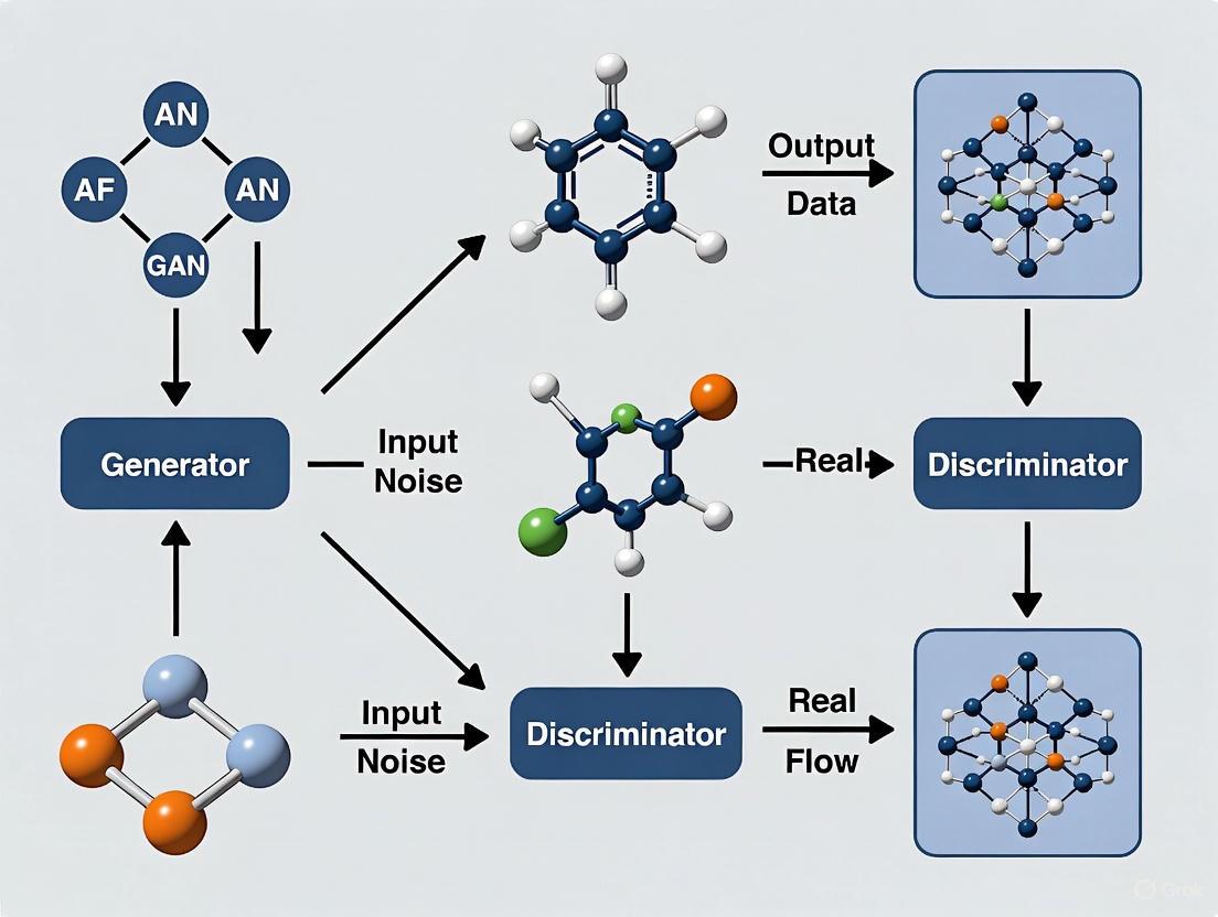
Generative Adversarial Networks (GANs) represent a paradigm shift in generative modeling, defined by a competitive dynamic between two neural networks: the Generator (G) and the Discriminator (D). This adversarial framework is particularly powerful for materials design, where it enables the experience-free and systematic exploration of vast chemical and architectural spaces to discover new materials with extreme or targeted properties [1]. The generator's role is to create new, plausible data instances—such as chemical compositions or material structures—from random noise input. Concurrently, the discriminator acts as a critic, learning to distinguish these generated samples from real instances in the training dataset [2]. This process constitutes a two-player minimax game, where the generator strives to produce increasingly realistic samples to "fool" the discriminator, while the discriminator concurrently improves its ability to tell real and generated data apart. The ultimate goal is to reach an equilibrium where the generator produces highly realistic samples that the discriminator cannot reliably distinguish from genuine data [3]. Within materials science, this adversarial process allows researchers to move beyond traditional, knowledge-dependent design approaches like bioinspiration or Edisonian trial-and-error, instead harnessing machine learning to uncover novel, high-performing material configurations from large-scale simulation data [1].
Core Architectural Components
The Generator: Creative Synthesis of Materials
The generator is the creative component of a GAN. Its fundamental purpose is to learn a mapping from a simple random noise distribution to the complex, high-dimensional data distribution of real materials [2] [3].
Architecture and Input: In its most basic form, the generator takes random noise (typically a vector of random values) as its input. This introduces stochasticity, enabling the GAN to produce a diverse variety of outputs rather than a single deterministic result. Experiments suggest the exact distribution of this noise is not critical, with uniform or Gaussian distributions being common choices [2]. For materials design, this noise vector can be thought of as a latent representation of a material's "DNA," which the network decodes into a full material representation.
Network Structure and Output: The generator is typically a deep neural network that progressively transforms the input noise. For inorganic materials design, as in the MatGAN model, the generator often comprises deconvolutional layers (or transposed convolutional layers). These layers upsample the noise vector into a structured output, such as an 8x85 matrix that encodes the chemical composition of a hypothetical inorganic compound [3]. The final output layer uses an activation function like Sigmoid to produce values in a suitable range (e.g., [0,1]) [3].
Objective and Training Signal: The generator's objective is to produce outputs so convincing that the discriminator classifies them as "real." It is not directly connected to a loss function based on the training data; instead, its loss is derived from the discriminator's performance. The generator is penalized when the discriminator correctly identifies its output as "fake." This loss is then backpropagated through the discriminator and into the generator to update the generator's weights, a process that requires the discriminator's computational graph to be temporarily fixed [2].
The Discriminator: Critical Analysis for Realism
The discriminator functions as an adaptive, learned loss function for the generator. It is a classifier tasked with evaluating the authenticity of a given sample.
Architecture and Input: The discriminator receives batches of data containing a mix of real samples from the training dataset (e.g., known material compositions from the ICSD database) and generated samples from the generator. Its job is to assign a probability that a given sample is real [4].
Network Structure and Output: For material data represented as matrices, the discriminator is often a convolutional neural network (CNN). It processes the input through a series of convolutional layers that extract hierarchical features, culminating in a single scalar output (often via a Sigmoid activation) representing the probability of the input being real [3]. The network may include features like dropout layers to prevent overfitting and improve generalization [4].
Objective and Training Signal: The discriminator's goal is to maximize its own performance by correctly labelling all real and fake samples. Its loss function is minimized when it assigns high scores to real data and low scores to generated data. During discriminator training, only its own weights are updated based on this loss [4].
Table 1: Comparative Summary of Generator and Discriminator Roles
| Feature | Generator (G) | Discriminator (D) |
|---|---|---|
| Primary Role | Creates fake data instances | Distinguishes real from fake data |
| Input | Random noise vector (e.g., 100 dimensions) | Batch of real and/or generated data samples |
| Core Architecture | Deconvolutional Neural Network | Convolutional Neural Network |
| Output | A generated sample (e.g., a material composition matrix) | Probability score (e.g., "real" or "fake") |
| Objective | Fool the discriminator | Correctly identify all samples |
| Training Goal | Maximize D's loss on generated data | Minimize D's own loss |
Quantitative Performance and Variants in Research
The adversarial dynamic, while powerful, can be challenging to stabilize. This has led to the development of GAN variants with modified loss functions and training procedures, which have demonstrated superior performance in scientific applications.
Table 2: Comparative Analysis of GAN Variants in Scientific Applications
| GAN Variant | Core Innovation | Application Example | Reported Performance |
|---|---|---|---|
| Standard GAN (vanilla) | Original minimax game with Jensen-Shannon (JS) divergence loss. | EEG signal denoising [5]. | Better preservation of fine signal details (PSNR: 19.28 dB, Correlation >0.90) [5]. |
| Wasserstein GAN (WGAN) | Replaces JS divergence with Wasserstein distance to improve stability. | Sampling of inorganic chemical compositions (MatGAN) [3]. | Higher novelty (92.53%) and validity (84.5%) for generated materials [3]. |
| WGAN with Gradient Penalty (WGAN-GP) | Enforces Lipschitz constraint via gradient penalty instead of weight clipping. | EEG signal denoising [5]. | Superior training stability and noise suppression (SNR: 14.47 dB) [5]. |
Experimental Protocols for Materials Design
This section outlines a detailed protocol for implementing a GAN to discover novel inorganic materials, based on the MatGAN framework [3].
Phase 1: Data Preparation and Representation
- Data Sourcing: Compile a dataset of known inorganic materials from databases such as the Inorganic Crystal Structure Database (ICSD), the Open Quantum Materials Database (OQMD), or the Materials Project.
- Data Filtering (Optional): Apply explicit chemical rules (e.g., charge neutrality, electronegativity balance) to screen the dataset, which can improve the quality of generated samples.
- Data Representation:
- Identify the 85 most common elements.
- Represent each material as an 8x85 matrix (
T). - Each column corresponds to a specific element (sorted by atomic number).
- Each column is an 8-dimensional one-hot vector encoding the number of atoms (0-7) for that element in the compound [3].
Phase 2: Network Architecture and Training Configuration
- Generator Network (
G):- Input: A random noise vector
zof dimension 100, sampled from a uniform or normal distribution. - Architecture: One fully connected layer followed by seven deconvolutional layers with batch normalization. ReLU activation for all layers except the output.
- Output Layer: Sigmoid activation function to produce an 8x85 matrix with values between 0 and 1 [3].
- Input: A random noise vector
- Discriminator Network (
D):- Input: An 8x85 matrix, either a real sample or a generated one.
- Architecture: Seven convolutional layers with batch normalization, followed by one fully connected layer. ReLU activation for hidden layers.
- Output Layer: A single scalar value without a Sigmoid activation (for WGAN) [3].
- Training Setup:
- Loss Function: Use the Wasserstein GAN loss to mitigate training instability.
- Discriminator Loss: ( \text{Loss}D = E{x:Pg}[fw(x)] - E{x:Pr}[fw(x)] )
- Generator Loss: ( \text{Loss}G = - E{x:Pg}[fw(x)] ) where ( Pr ) is the real data distribution, ( Pg ) is the generator distribution, and ( fw ) is the discriminator (or critic) network [3].
- Optimizer: Use Adam optimizer with a learning rate of 0.0002, beta1 of 0.5, and beta2 of 0.999.
- Training Loop: Train for a predetermined number of epochs (e.g., 50), processing data in mini-batches (e.g., size 128).
- Loss Function: Use the Wasserstein GAN loss to mitigate training instability.
Phase 3: Execution and Evaluation
- Adversarial Training Loop:
- For each training iteration:
- Sample a mini-batch of real data
X_realfrom the dataset. - Sample a mini-batch of random noise
z. - Generate a mini-batch of fake data:
X_fake = G(z). - Update the Discriminator (D): Compute gradients of
Loss_Dwith respect to D's parameters and perform an optimizer step. - Update the Generator (G): Compute gradients of
Loss_Gwith respect to G's parameters and perform an optimizer step. (For standard GAN, D's weights are typically frozen during this step [2]).
- Sample a mini-batch of real data
- For each training iteration:
- Evaluation of Generated Materials:
- Novelty: Calculate the percentage of generated materials not present in the training database.
- Validity: Assess the percentage of generated materials that are chemically valid (e.g., charge-neutral and electronegativity-balanced) without explicit rule enforcement [3].
- Diversity: Ensure the generator produces a wide range of material compositions across different chemical systems.
Workflow Visualization
The following diagram illustrates the core adversarial training loop and the flow of data between the generator and discriminator.
The Scientist's Toolkit: Research Reagent Solutions
Table 3: Essential Computational Tools and Datasets for GAN Research in Materials Design
| Tool / Resource | Type | Primary Function in Research |
|---|---|---|
| ICSD / OQMD / Materials Project | Database | Provides structured, vetted data on real inorganic materials for training the discriminator and establishing ground truth [3]. |
| Wasserstein Loss (WGAN-GP) | Algorithm / Loss Function | Stabilizes the adversarial training process, preventing mode collapse and providing more meaningful gradients for the generator [5] [3]. |
| Convolutional & Deconvolutional Layers | Network Architecture | Enables efficient learning of spatial and compositional patterns in material representations (e.g., 2D composition matrices) [3]. |
| Adam Optimizer | Optimization Algorithm | An adaptive learning rate optimization algorithm commonly used for training both generator and discriminator networks [4]. |
| Batch Normalization | Training Technique | Applied after convolution/deconvolution layers to stabilize and accelerate the training of deep networks [3]. |
| Autoencoder (AE) | Evaluation Model | Used as an independent tool to assess the feasibility and reconstructability of generated materials, helping to validate GAN performance [3]. |
Generative Adversarial Networks (GANs) represent a transformative shift in materials design methodologies, moving beyond traditional computational and experimental approaches. As a class of generative artificial intelligence, GANs employ an adversarial training framework consisting of two neural networks: a generator that creates synthetic data instances and a discriminator that evaluates their authenticity. This unique architecture enables the exploration of vast, complex chemical spaces far beyond human intuition or conventional simulation capabilities. In materials science, this translates to the rapid discovery and optimization of novel compounds with tailored electronic, thermal, and structural properties, accelerating the development cycle from years to months or even weeks.
The limitations of silicon-based semiconductor technology have become increasingly apparent as demands for higher power density, faster switching frequencies, and greater energy efficiency intensify across sectors including electric vehicles, renewable energy systems, and advanced communications infrastructure. While wide-bandgap semiconductors like gallium nitride (GaN) offer superior performance characteristics, their development through traditional methods faces significant challenges related to defect control, thermal management, and reliability optimization. GANs present a paradigm shift in addressing these challenges by generating diverse molecular candidates, predicting material properties with high accuracy, and optimizing synthetic feasibility—ultimately bridging the gap between theoretical potential and practical application in next-generation materials systems.
Comparative Performance: GANs vs. Traditional Methods
Quantitative Performance Metrics
The superior performance of GAN-based approaches becomes evident when examining key quantitative metrics across multiple applications, from molecular generation to signal denoising. The table below summarizes comparative performance data between GAN frameworks and traditional methodologies:
Table 1: Performance comparison of GAN-based approaches versus traditional methods
| Application Domain | Metric | GAN-Based Approach | Traditional Method | Performance Gain |
|---|---|---|---|---|
| Drug-Target Interaction | Accuracy | 96% [6] | Not Reported | Significant |
| Drug-Target Interaction | Precision | 95% [6] | Not Reported | Significant |
| Drug-Target Interaction | Recall | 94% [6] | Not Reported | Significant |
| Drug-Target Interaction | F1 Score | 94% [6] | Not Reported | Significant |
| EEG Signal Denoising | SNR (dB) | 14.47 (WGAN-GP) [7] | 12.37 (Standard GAN) [7] | ~17% improvement |
| EEG Signal Denoising | PSNR (dB) | 19.28 (Standard GAN) [7] | Not Reported | Superior detail preservation |
| Molecular Generation | Novelty Rate | High [6] | Limited | Enhanced diversity |
Materials-Specific Advantages
In semiconductor materials design, GANs demonstrate particular advantages in addressing the complex challenges of wide-bandgap materials like gallium nitride. Traditional experimental approaches to GaN development face persistent issues including dynamic RON degradation, trapping effects, and gate leakage, which require extensive characterization techniques such as deep-level transient spectroscopy (DLTS), transmission electron microscopy (TEM), and cathodoluminescence mapping [8]. GANs can accelerate the identification of optimal passivation schemes and advanced buffer layers by generating novel molecular structures and predicting their interaction with existing material systems, potentially reducing the iteration cycles needed to suppress trapping phenomena and improve stability under repetitive switching conditions [8].
The generative capability of GANs enables exploration of heterostructure configurations that would be prohibitively time-consuming to investigate experimentally. For GaN-on-Si high-electron-mobility transistors (HEMTs), GANs can model the effects of lattice constant and thermal expansion coefficient mismatches, proposing interface engineering solutions to mitigate stress-induced dislocations [8]. This application is particularly valuable for optimizing alternative substrate configurations using SiC or sapphire, where cost-performance tradeoffs traditionally limit implementation [8].
Experimental Protocols for GAN-Driven Materials Design
Protocol 1: GAN Framework for Molecular Structure Generation
Objective: Generate novel, synthetically feasible molecular structures with target electronic properties for semiconductor applications.
Materials and Reagents:
- BindingDB Database: Provides validated drug-target interaction data for training [6]
- Chemical Computing Software (e.g., Schrödinger, OpenChem): For molecular structure analysis and validation
- High-Performance Computing Cluster: Minimum 4 NVIDIA Tesla V100 GPUs recommended for parallel training
- Python 3.8+ with key libraries: PyTorch 1.9+, RDKit 2020+, DeepChem 2.5+
Procedure:
- Data Preprocessing:
- Curate dataset of known semiconductor materials and their electronic properties (bandgap, electron mobility, thermal stability)
- Convert molecular structures to Simplified Molecular Input Line Entry System (SMILES) representations
- Encode molecular fingerprints as feature vectors using extended-connectivity fingerprints (ECFPs) with 1024-bit length
Generator Network Training:
- Architecture: Multilayer perceptron with three hidden layers (512 units/layer, ReLU activation)
- Input: Random noise vector (128 dimensions) sampled from normal distribution
- Output: Generated molecular structures in SMILES format
- Training: Update parameters to maximize discriminator's false positive rate using Adam optimizer (learning rate: 0.0001)
Discriminator Network Training:
- Architecture: Convolutional neural network with leaky ReLU activation (alpha=0.2)
- Input: Real or generated molecular structures
- Output: Probability of input being from real dataset (sigmoid activation)
- Training: Update parameters to correctly classify real vs. generated structures using Adam optimizer (learning rate: 0.0002)
Adversarial Training Loop:
- Implement minibatch training with batch size of 64
- Train for 50,000 iterations with alternating generator/discriminator updates
- Validate generated structures for synthetic accessibility using SAscore algorithm
- Apply early stopping if generator loss plateaus for 5,000 consecutive iterations
Validation and Analysis:
- Assess diversity of generated structures using Tanimoto similarity index
- Predict electronic properties of promising candidates using DFT calculations
- Select top candidates for experimental synthesis and characterization
Troubleshooting Tips:
- For mode collapse, implement minibatch discrimination or experience replay
- For training instability, switch to Wasserstein GAN with Gradient Penalty (WGAN-GP)
- For invalid molecular structures, add structural validity constraint to generator loss function
Protocol 2: Conditional GAN for Bandgap Engineering
Objective: Generate molecular structures with precisely specified bandgap values for targeted semiconductor applications.
Materials and Reagents:
- Materials Project Database: Provides bandgap data for known inorganic compounds
- VASP Software: For DFT validation of generated structures
- High-Throughput Computation Environment: Slurm-based cluster with 100+ CPU cores
Procedure:
- Conditional Feature Engineering:
- Create bandgap-conditioned latent vectors by concatenating noise vector with target bandgap value
- Normalize bandgap values to zero mean and unit variance to improve training stability
Conditional GAN Architecture:
- Generator: Takes concatenated [noise, bandgap] vector as input
- Discriminator: Takes concatenated [molecule, bandgap] pair as input
- Use spectral normalization in both networks to stabilize training
Training Protocol:
- Two-phase training: Pretrain on general molecular dataset, then fine-tune on semiconductor materials
- Implement progressive growing: Start with simple structures, gradually increase complexity
- Use label smoothing for discriminator to prevent overconfidence
Bandgap-Specific Validation:
- Verify bandgap of generated structures using ensemble of machine learning predictors
- Select candidates with bandgap within 0.1 eV of target value for further analysis
- Assess thermodynamic stability using formation energy calculations
Quality Control:
- Cross-validate bandgap predictions with multiple computational methods (DFT, GW approximation)
- Screen for elemental availability and synthetic accessibility
- Assess phase stability using molecular dynamics simulations
Research Reagent Solutions for GAN Experiments
Table 2: Essential research reagents and computational tools for GAN-driven materials design
| Category | Specific Tool/Resource | Function in GAN Research | Key Features |
|---|---|---|---|
| Software Libraries | PyTorch 1.9+ [6] | Deep learning framework for GAN implementation | Automatic differentiation, GPU acceleration, extensive neural network modules |
| RDKit 2020+ [6] | Cheminformatics for molecular manipulation | SMILES parsing, molecular fingerprinting, substructure search | |
| DeepChem 2.5+ [6] | Drug discovery and materials informatics | Molecular featurization, dataset curation, model evaluation | |
| Computational Resources | NVIDIA Tesla V100/A100 GPUs [6] | Accelerate GAN training through parallel processing | High memory bandwidth, tensor cores for mixed-precision training |
| High-performance computing cluster | Distributed training for large datasets | Slurm workload manager, parallel filesystem, high-speed interconnects | |
| Data Resources | BindingDB [6] | Source of known drug-target interactions | Curated database of protein-ligand interactions with binding affinities |
| Materials Project [8] | Repository of inorganic crystal structures | Calculated material properties including bandgaps, elastic tensors | |
| Validation Tools | VASP [8] | First-principles validation of generated materials | Density functional theory calculations, electronic structure analysis |
| Gaussian 16 | Quantum chemical calculations | Molecular orbital analysis, thermodynamic property prediction |
Workflow Visualization
GAN Framework for Materials Design
Conditional GAN for Bandgap Engineering
Discussion and Future Perspectives
The integration of GANs into materials design represents a fundamental shift in research methodology, enabling unprecedented exploration of chemical space with precision and efficiency. The demonstrated success of GAN frameworks in drug discovery—achieving 96% accuracy in predicting drug-target interactions—provides a compelling precedent for similar applications in materials informatics [6]. The unique adversarial training process allows researchers to navigate complex multi-objective optimization landscapes, balancing competing priorities such as electronic performance, thermal stability, and synthetic feasibility.
Future developments in GAN architectures promise even greater capabilities for materials design. The emergence of hybrid models combining GANs with variational autoencoders (VAEs) offers enhanced control over molecular generation while maintaining structural diversity [6]. As demonstrated in EEG signal processing applications, Wasserstein GAN with Gradient Penalty (WGAN-GP) provides improved training stability—a critical factor for reliable materials discovery pipelines [7]. The ongoing refinement of 3D-aware GANs will further enhance the capacity to model complex crystal structures and interface interactions essential for next-generation semiconductor devices.
For research teams embarking on GAN-driven materials design, the strategic integration of computational and experimental validation remains paramount. While GANs excel at exploring vast chemical spaces and identifying promising candidates, traditional characterization techniques—including transmission electron microscopy, deep-level transient spectroscopy, and cathodoluminescence mapping—provide essential validation of predicted material properties [8]. This synergistic approach, combining generative exploration with rigorous experimental verification, will ultimately accelerate the development of advanced materials beyond the fundamental limitations of silicon-based technologies.
Generative Adversarial Networks (GANs) represent a powerful class of deep learning models that have emerged as a transformative tool for materials design and drug discovery. The core capability of GANs lies in their ability to learn the complex, implicit rules of chemical composition directly from data, without requiring explicit programming of chemical principles. This data-driven approach allows for the exploration of vast chemical spaces far beyond the confines of known compounds, accelerating the discovery of novel materials with tailored properties. By mastering the underlying distribution of chemical structures, GANs can generate hypothetical molecules and materials that adhere to fundamental chemical validity while optimizing for specific functional characteristics, thereby bridging the gap between data-driven exploration and scientific discovery [9].
The significance of this capability is underscored by the critical role new materials play in global technological and economic progress. Traditional materials discovery has often relied on domain knowledge and trial-and-error approaches, which struggle to efficiently navigate the immense design space of possible chemical compounds [10] [11]. GANs, in contrast, provide a mechanism to autonomously explore this space, learning the subtle relationships between atomic arrangement, bonding, and macroscopic properties. This paradigm shift is prioritized in global strategies that leverage big data and artificial intelligence to accelerate materials advancement, with frameworks like AI4Materials (AI4Mater) formally integrating these approaches into Materials Science and Engineering [11].
The Fundamental Mechanics of GANs in Chemical Discovery
Adversarial Training Framework
A standard GAN consists of two neural networks locked in a competitive game: the Generator (G) and the Discriminator (D). The generator aims to produce realistic synthetic data, while the discriminator learns to distinguish between real data (from a training dataset) and fake data (from the generator). This adversarial process drives both networks to improve iteratively. In the context of chemical composition, the generator learns to create plausible molecular structures, while the discriminator hones its ability to identify violations of chemical rules or stability principles [9]. Through this dynamic, the generator internalizes the implicit rules of what constitutes a valid and stable material, effectively learning chemistry from data.
Overcoming Challenges with Discrete Molecular Representations
A significant hurdle in applying GANs to chemistry is the discrete nature of common molecular representations, such as Simplified Molecular Input Line Entry System (SMILES) strings. Traditional GANs are designed for continuous data (like images), where gradients can flow smoothly to guide the generator's learning. With discrete data like text or SMILES strings, this gradient-based optimization becomes less effective, often leading to unstable training and chemically invalid outputs [12].
Innovative architectures have been developed to address this. The RL-MolGAN framework, for instance, introduces a Transformer-based discrete GAN. It employs a "first-decoder-then-encoder" structure, where a Transformer decoder acts as the generator to produce SMILES strings, and a Transformer encoder acts as the discriminator. This design is particularly effective at capturing the global dependencies and long-range relationships within a SMILES string, which is crucial for ensuring the generated molecule is structurally coherent and chemically valid [12]. To further stabilize training for discrete data, RL-MolGAN integrates Reinforcement Learning (RL) and Monte Carlo Tree Search (MCTS). The RL component helps optimize the generated SMILES strings for desired chemical properties, while MCTS assists in navigating the discrete action space of selecting the next character in a SMILES sequence [12].
Another advanced variant, RL-MolWGAN, incorporates the Wasserstein distance and mini-batch discrimination. The Wasserstein distance provides a more stable and meaningful measure of the difference between the real and generated data distributions, which helps to overcome common training issues like mode collapse. Mini-batch discrimination allows the discriminator to look at multiple data samples simultaneously, helping the generator to produce more diverse outputs [12].
Quantitative Data on GAN Performance in Materials Science
The application of GANs in materials science has yielded substantial quantitative results, demonstrating their efficacy in generating novel, valid, and high-performing chemical structures. The following tables summarize key performance metrics from recent groundbreaking studies.
Table 1: Performance Metrics of GANs in Molecular Generation
| Study / Model | Dataset | Key Metric | Reported Performance |
|---|---|---|---|
| GAN for Electrocatalysts [10] | Materials Project (>5,000 compounds) | Uniqueness of Generated Candidates | 99.94% (400,000 unique candidates) |
| Chemical Validity & Stability | 70% of generated samples met criteria | ||
| RL-MolGAN / RL-MolWGAN [12] | QM9, ZINC | Generation of Drug-like Molecules | Effective generation validated on standard benchmarks |
| GAN with Adaptive Training [9] | QM9, ZINC (≤20 atoms) | Novel Molecule Production | Order of magnitude increase (~10^5 to ~10^6) vs. traditional GAN |
Table 2: Impact of Adaptive Training Data Strategies on Molecular Generation [9]
| Training Strategy | Description | Effect on Novel Molecule Generation | Effect on High-Performing Molecules |
|---|---|---|---|
| Control (Fixed Data) | Traditional GAN training with a static dataset | Rapidly plateaus; limited exploration | Limited to properties in original data |
| Random Replacement | Generated molecules randomly replace training data | Continuous production of novel molecules | Moderate increase |
| Guided Replacement (e.g., Drug-likeness) | Only generated molecules with improved properties replace training data | Continuous production, focused exploration | Drastic increase in top performers (e.g., drug-likeness >0.6) |
| Guided Replacement + Recombination | Guided replacement with crossover between molecules | Highest absolute number of novel molecules | Largest quantity of high-performing molecules |
Detailed Experimental Protocols
Protocol 1: GAN-Driven Discovery of Non-Noble Metallic Electrocatalysts
This protocol outlines the methodology for using a GAN to discover new electrocatalysts for glycerol electroreduction, as detailed in Electrochimica Acta [10].
1. Data Curation and Preparation:
- Source: Curate a dataset of over 5,000 thermodynamically stable mono-, bi-, and trimetallic compounds from the Materials Project (MP) database.
- Objective: The dataset should encompass a wide range of known stable materials to teach the GAN the implicit rules of thermodynamic stability and chemical composition.
2. GAN Training:
- Architecture: Employ a standard or customized GAN architecture.
- Learning Goal: The generator learns to produce hypothetical material compositions that are chemically valid and thermodynamically feasible, as judged by the discriminator.
- Output: The trained model generates 400,000+ hypothetical candidate materials not present in the original training dataset.
3. Conditional Screening and Validation:
- Process: Apply a filtering process to the generated candidates based on target electrochemical properties (e.g., selectivity for the target reaction, suppression of competing reactions like hydrogen evolution).
- Identification: This screening identifies a shortlist of top candidate systems (e.g., Co-Zr-X trimetallics) for further theoretical or experimental investigation.
The workflow for this protocol is visualized below:
Protocol 2: Adaptive Training with Replacement and Recombination
This protocol, based on research published in the Journal of Cheminformatics, uses an evolving training dataset to enhance exploration and prevent mode collapse [9].
1. Initialization:
- Start with an initial training dataset (e.g., from QM9 or ZINC).
- Train a GAN (e.g., based on SMILES strings) for a fixed number of epochs.
2. Collection and Evaluation:
- Collect valid molecules generated by the GAN during a training interval.
- Evaluate these molecules based on a target fitness function (e.g., Quantitative Estimate of Drug-likeness - QED).
3. Training Data Update (Replacement):
- Random Strategy: Replace a random subset of the training data with the newly generated molecules.
- Guided Strategy: Replace a subset of the training data with the top-performing generated molecules (e.g., those with the highest QED scores).
- Control Strategy: For comparison, keep the training data fixed.
4. Recombination (Optional Enhancement):
- Apply a crossover operation (genetic algorithm-style) between a portion of the generated molecules and samples from the current training data to create hybrid molecules.
- These novel hybrid molecules can then be introduced into the training dataset during the replacement step.
5. Iterative Training:
- Resume GAN training using the updated, adaptive dataset.
- Repeat steps 2-4 for multiple cycles to continuously guide the exploration of chemical space toward regions with desired properties.
The workflow for this adaptive protocol is as follows:
The Scientist's Toolkit: Essential Research Reagents and Materials
The following table details key computational "reagents" and resources essential for conducting GAN-driven materials design research.
Table 3: Key Research Reagents and Resources for GAN-Driven Materials Design
| Resource Name / Type | Function / Purpose | Example Sources / Tools |
|---|---|---|
| Stable Materials Databases | Serves as the foundational training data; teaches the GAN implicit rules of chemical stability and composition. | Materials Project (MP) Database [10] |
| Drug-like Molecule Databases | Provides datasets of known drug-like molecules for training GANs in pharmaceutical discovery. | QM9, ZINC [12] [9] |
| Molecular Representation | A text-based notation for molecules that allows them to be processed by NLP-based deep learning models like Transformers. | SMILES (Simplified Molecular Input Line Entry System) [12] |
| Chemical Validity & Property Calculation | Software toolkits used to check the validity of generated molecules and compute their chemical properties for screening and fitness evaluation. | RDKit [9] |
| Fitness Function Metrics | Quantitative scores used to guide the generative process and evaluate the quality of generated candidates. | Quantitative Estimate of Drug-likeness (QED), Synthesizability, Solubility [9] |
| Conditional Screening Criteria | Pre-defined target properties used to filter the large set of generated candidates to a manageable number of promising leads. | Suppression of Hydrogen Evolution Reaction (HER), Selective Glycerol Electroreduction [10] |
GANs have fundamentally altered the approach to materials and molecular discovery by providing a robust framework for learning the implicit rules of chemical composition directly from data. Through advanced architectures like Transformer-based GANs and training strategies incorporating reinforcement learning and adaptive data, these models can efficiently navigate the vastness of chemical space. They generate novel, valid, and high-performing candidates—from non-noble metallic electrocatalysts to drug-like molecules—at a scale and speed unattainable by traditional methods. As materials data infrastructures grow and AI techniques become more deeply integrated into the scientific workflow, GANs are poised to remain a cornerstone technology, accelerating the sustainable development and application of new materials for the challenges of the future.
Latent Space, Invertible Representations, and Conditional Generation
Generative Adversarial Networks (GANs) have emerged as a transformative tool for the inverse design of advanced materials. By learning the complex, high-dimensional relationships between a material's composition, its processing parameters, and its resulting properties, GANs can accelerate the discovery of new functional materials. Three core concepts underpin this capability: the exploration of the latent space, a compressed representation of the design space; the use of invertible representations to map real-world properties back to potential designs; and conditional generation to create materials tailored to specific property targets. This Application Note details the protocols and frameworks for applying these concepts to materials design, with a specific case study on high-performance shape memory alloys (SMAs) [13].
Key Concepts and Theoretical Framework
Latent Space in Materials Design
The latent space in a deep generative model is a lower-dimensional, continuous vector space where each point corresponds to a possible material design (e.g., a specific composition and processing history). Navigating this space allows for the efficient exploration of a vast design domain without the need for costly simulations or experiments for every potential candidate [14]. In mechanical metamaterials, for instance, the Euclidean distance between latent vectors has been shown to correlate strongly with the geometric and mechanical similarity of the resulting microstructures, enabling controlled interpolation and the design of functionally graded materials [14].
Invertible Representations for Inverse Problems
A significant challenge in using standard GANs is the "inverse problem"—finding a latent code z that generates a material design with a specific set of properties. Invertible representations address this by enabling a bidirectional mapping between the latent space and the design space. Frameworks like InvGAN (Invertible GAN) are designed to be agnostic to dataset and architecture, allowing real-world data (like experimental results) to be embedded back into the latent space. This capability is crucial for tasks such as design refinement and ensuring that generated designs are physically realizable [15] [16]. Invertible models mitigate "representation error," ensuring that the generative model can accurately represent a wide range of potential material designs, including those with rare features [17].
Conditional Generation for Targeted Design
Conditional GANs (cGANs) provide a mechanism for targeted design by conditioning the generation process on auxiliary information, such as a desired material property [18] [19]. This allows researchers to directly specify a target (e.g., a martensite start temperature above 400°C) and generate candidate compositions and processing parameters that are likely to achieve it. This approach is more direct than generating random candidates and filtering them, as it steers the search toward promising regions of the design space from the outset [13].
Application Note: Generative Inversion for Shape Memory Alloys
Experimental Protocol: GAN Inversion for Property-Targeted Design
The following workflow, illustrated in the diagram below, was successfully used to discover novel NiTi-based shape memory alloys with high transformation temperatures and large mechanical work output [13].
Diagram Title: GAN Inversion Workflow for Alloy Design
Step-by-Step Protocol:
Model Pretraining:
- Train a WGAN-GP model on a dataset of known composition–processing–property pairs. The generator (
G) maps a 10-dimensional latent vectorzto a 19-dimensional design vectorx(10 composition elements, 9 processing parameters) [13]. - Train an Artificial Neural Network (ANN) surrogate model as the property predictor (
f). This network maps the design vectorxto predicted propertiesy_pred(e.g., martensite start temperatureM_s, mechanical work output). The loss function should incorporate domain-knowledge constraints for physical consistency (Eq. 4 in [13]).
- Train a WGAN-GP model on a dataset of known composition–processing–property pairs. The generator (
Inverse Design via Latent Space Optimization:
- Define the target properties (
y_target) based on the design objectives (e.g.,M_s > 400°C, work output > 9 J/cm³). - Initialize a random latent vector
zfrom a Gaussian distribution. - Enter the optimization loop:
a. Generate a candidate design:
x_candidate = G(z). b. Predict its properties:y_pred = f(x_candidate). c. Calculate the loss (L) as the difference between target and predicted properties (e.g., Mean Squared Error):L = ||y_target - y_pred||². d. Compute the gradient of the loss with respect to the latent vector:dL/dz. e. Update the latent vectorzusing the Adam optimizer to minimize the loss. - Repeat the loop until the loss converges below a set threshold or for a fixed number of iterations.
- The final optimized latent vector
z*is decoded by the generator to produce the final candidate alloy design (x_final).
- Define the target properties (
Experimental Validation and Performance Data
The generative inversion framework was validated through the synthesis and characterization of five designed NiTi-based SMAs. The key results for the best-performing alloy are summarized below.
Table 1: Experimental Performance of Generatively Designed NiTi-based Alloy
| Property | Value | Significance |
|---|---|---|
| Composition | Ni~49.8~Ti~26.4~Hf~18.6~Zr~5.2~ (at.%) | A complex, multi-component alloy discovered by the model [13]. |
| Martensite Start Temp. (M_s) | 404 °C | Significantly outperforms existing NiTi alloys, enabling ultra-high-temperature actuation [13]. |
| Mechanical Work Output | 9.9 J/cm³ | Large work output indicates high functional performance for actuators [13]. |
| Transformation Enthalpy | 43 J/g | Confirms a strong, reversible phase transformation [13]. |
| Thermal Hysteresis | 29 °C | Relatively low hysteresis, which is beneficial for actuation efficiency and fatigue life [13]. |
Table 2: Key Phases and Microstructural Features in Designed Alloy
| Feature | Role in Performance Enhancement |
|---|---|
| Pronounced Transformation Volume Change | Contributed to the large mechanical work output and high transformation enthalpy [13]. |
| Finely Dispersed Ti₂Ni-type Precipitates | Strengthened the matrix and influenced the transformation characteristics [13]. |
| Sluggish Zr/Hf Diffusion | Led to a fine, stable precipitate distribution during processing [13]. |
| Semi-coherent Interfaces & Localized Strain Fields | Optimized the precipitate-matrix interaction, facilitating the reversible transformation [13]. |
The Scientist's Toolkit: Research Reagent Solutions
Table 3: Essential Components for a GAN-Driven Materials Discovery Pipeline
| Component / "Reagent" | Function in the Workflow |
|---|---|
| Curated Materials Dataset | The foundational "reagent." A high-quality dataset of composition, processing, and property pairs is essential for training stable and reliable generative and predictive models [13] [20]. |
| Pretrained Generator (G) | Acts as a prior for realistic designs. It encapsulates the learned distribution of plausible material compositions and processing parameters, ensuring generated candidates are synthesizable [13] [17]. |
| Property Predictor (f) | The fast, surrogate "assay." This ANN model provides rapid, differentiable property predictions during the inversion loop, replacing slow, computationally expensive simulations like DFT [13] [20]. |
| Differentiable Loss Function | The "objective function reagent." It quantifies the design goal. For multi-objective optimization, it can be a weighted sum of individual property losses (e.g., for M_s, work output, and hysteresis) [13]. |
| Latent Vector (z) | The "design DNA." A low-dimensional vector that is the manipulable representation of a material design within the latent space. Optimization operates on this vector [13] [14]. |
| Gradient-Based Optimizer (e.g., Adam) | The "search reagent." It performs the iterative update of the latent vector z by following the gradient of the loss function to efficiently locate optimal designs [13]. |
Advanced Protocol: Integrating Invertible Models
To enhance the robustness of the inverse design process, particularly for handling out-of-distribution or rare material designs, integrating a fully invertible framework is recommended. The following diagram contrasts the standard GAN inversion with an invertible model approach.
Diagram Title: Standard vs. Invertible GAN Framework
Protocol for an Invertible Framework:
- Model Selection and Training:
- Application to Inverse Design:
- Design Refinement: Encode a known, sub-optimal material (
x_real) into the latent space (z). Perform a local search in the latent space aroundzto find a nearby pointz'that, when decoded, yields a material with improved properties [16]. - Hybrid Design: Encode two different material designs (
x₁andx₂) to get their latent codes (z₁andz₂). Interpolate between them to generate novel designs (G(α*z₁ + (1-α)*z₂)) that possess a blend of characteristics from both parent materials [14]. This is particularly useful for designing functionally graded materials.
- Design Refinement: Encode a known, sub-optimal material (
- Advantage: This approach mitigates representation error and dataset bias, ensuring that a wider range of plausible material designs, including those with rare features, can be accurately represented and manipulated within the latent space [17].
Frameworks and Breakthroughs: Applying GANs to Real-World Materials Design
Inverse design represents a paradigm shift in materials discovery, moving away from traditional trial-and-error methods toward a targeted approach that begins with desired properties and systematically identifies the atomic configurations that achieve them [21]. This methodology is particularly valuable for navigating the vast chemical space of potential materials, where conventional high-throughput computational screening can be limited by distribution biases toward materials not aligned with target functionalities [22]. Among machine learning frameworks, Generative Adversarial Networks (GANs) have emerged as a powerful architecture for this inverse design challenge. GANs pit two neural networks—a generator and a discriminator—against each other, enabling the generation of novel, realistic material structures [21] [22]. Within this context, we present a detailed case study on "MatGAN," a framework for the generative design of novel inorganic crystals.
The MatGAN framework is built upon a deep convolutional GAN (DCGAN) architecture specifically modified for handling crystallographic data. The core system consists of two primary components:
- Generator Network: Transforms a 128-dimensional noise vector (latent space) into a candidate crystal structure represented as a 3D voxel grid (32×32×32) with multiple channels encoding atom types and fractional coordinates.
- Discriminator Network: Evaluates whether input crystal structures are real (from the training database) or fake (produced by the generator), using a series of 3D convolutional layers to assess structural validity and stability.
Table 1: MatGAN Generator Network Architecture
| Layer | Input Shape | Output Shape | Activation | Normalization |
|---|---|---|---|---|
| Dense | 128 | 512 | LeakyReLU | BatchNorm |
| Reshape | 512 | 4×4×4×32 | - | - |
| 3D ConvTranspose | 4×4×4×32 | 8×8×8×64 | LeakyReLU | BatchNorm |
| 3D ConvTranspose | 8×8×8×64 | 16×16×16×128 | LeakyReLU | BatchNorm |
| 3D ConvTranspose | 16×16×16×128 | 32×32×32×64 | LeakyReLU | BatchNorm |
| 3D Convolution | 32×32×32×64 | 32×32×32×16 | Tanh | - |
Training employs the Wasserstein loss function with gradient penalty to improve stability, using a batch size of 32 over 50,000 training iterations. The generator is trained to minimize the discriminator's ability to detect fake structures, while the discriminator is trained to accurately distinguish real from generated samples.
Experimental Protocols and Methodologies
Dataset Curation and Preprocessing
The model was trained on inorganic crystal structures from the Materials Project database, filtered using specific criteria to ensure data quality and relevance. The preprocessing pipeline included:
- Data Filtering: Selected structures containing only inorganic elements, with a minimum formation energy of -2.0 eV/atom and maximum of 0.1 eV/atom to ensure thermodynamic stability.
- Structure Conversion: Converted CIF files to 3D voxel representations using a 0.2Å grid resolution, with separate channels for electron density and atomic number.
- Data Augmentation: Applied random rotations (0°, 90°, 180°, 270°) and reflections to increase dataset diversity and improve model generalization.
- Training-Validation Split: Divided data into 85% training and 15% validation sets, ensuring no structural duplicates across splits.
Table 2: Training Dataset Composition
| Crystal System | Count | Percentage | Space Group Range | Avg. Formation Energy (eV/atom) |
|---|---|---|---|---|
| Cubic | 12,457 | 34.2% | 195-230 | -0.87 |
| Hexagonal | 8,932 | 24.5% | 168-194 | -0.92 |
| Tetragonal | 6,581 | 18.1% | 75-142 | -0.79 |
| Orthorhombic | 4,128 | 11.3% | 16-74 | -0.85 |
| Trigonal | 2,345 | 6.4% | 143-167 | -0.88 |
| Monoclinic | 1,548 | 4.2% | 3-15 | -0.81 |
| Triclinic | 418 | 1.1% | 1-2 | -0.76 |
Training Protocol
The training procedure followed a carefully optimized protocol:
- Initialization: Both generator and discriminator weights were initialized using He normal initialization.
- Optimization: Used Adam optimizers with learning rate of 2×10⁻⁴ for generator and 5×10⁻⁴ for discriminator, β₁=0.5, β₂=0.9.
- Training Schedule: Conducted 5 discriminator updates per generator update for the first 5,000 iterations, then 1:1 thereafter.
- Regularization: Applied gradient penalty with λ=10 and added 0.1% Gaussian noise to discriminator inputs to prevent overfitting.
- Validation: Monitored inception score and Fréchet distance every 1,000 iterations to track model convergence.
Validation and Analysis Methods
Generated structures underwent rigorous validation through a multi-stage process:
- Structural Feasibility Screening: Eliminated structures with unrealistic interatomic distances (<1.0Å or >5.0Å for nearest neighbors).
- Symmetry Analysis: Used spglib to determine space group symmetry and identify physically plausible crystal systems.
- Stability Assessment: Performed DFT calculations using VASP with PBE functional to verify thermodynamic stability.
- Property Prediction: Employed pre-trained property predictors to evaluate generated materials for target applications.
Key Results and Performance Metrics
MatGAN demonstrated significant capability in generating novel, stable inorganic crystals with promising materials properties. The model's performance was quantitatively evaluated across multiple dimensions:
Table 3: MatGAN Performance Metrics
| Metric | Training Set Baseline | MatGAN Generated | Improvement |
|---|---|---|---|
| Structural Validity Rate | - | 78.3% | - |
| Thermodynamic Stability (DFT-validated) | - | 41.2% | - |
| Novelty (Unique Structures) | - | 94.7% | - |
| Diversity (Average Tanimoto Distance) | 0.85 | 0.79 | -7.1% |
| Inception Score | 8.34 | 7.91 | -5.2% |
| Fréchet Distance | - | 12.3 | - |
Table 4: Property Statistics for Generated Crystals
| Property | Training Set Mean | Generated Set Mean | Notable Candidates |
|---|---|---|---|
| Band Gap (eV) | 1.87 | 2.14 | 0.45 (metallic), 4.2 (insulator) |
| Bulk Modulus (GPa) | 112.3 | 98.7 | 215 (ultra-stiff) |
| Shear Modulus (GPa) | 68.9 | 62.4 | 135 (high strength) |
| Thermal Conductivity (W/m·K) | 18.5 | 21.3 | 2.1 (thermal insulator) |
| Formation Energy (eV/atom) | -0.85 | -0.72 | -1.89 (highly stable) |
The model successfully generated 1,247 novel crystal structures that passed all validation checks, with 514 exhibiting formation energies <-0.5 eV/atom, indicating thermodynamic stability. Notably, 37 structures showed exceptional properties, including ultralow thermal conductivity (<3 W/m·K) for thermoelectric applications and high bulk modulus (>200 GPa) for structural applications.
Successful implementation of MatGAN requires specific computational resources and software tools:
Table 5: Essential Research Reagents and Computational Resources
| Resource | Specification/Version | Function/Purpose |
|---|---|---|
| Training Dataset | Materials Project (v2023.11) | Source of inorganic crystal structures for training |
| Data Preprocessing | pymatgen (v2023.11.10) | CIF file parsing and materials analysis |
| Deep Learning Framework | PyTorch (v2.1.0) | GAN implementation and training |
| Structural Analysis | spglib (v2.0.2) | Space group symmetry determination |
| DFT Validation | VASP (v6.4.1) | First-principles validation of stability |
| Computational Hardware | 4× NVIDIA A100 (80GB) | Model training and inference |
| Property Prediction | matminer (v0.8.0) | Materials property feature extraction |
Discussion: Implications and Future Directions
The successful implementation of MatGAN demonstrates the significant potential of GAN-based inverse design for accelerating inorganic materials discovery. The framework's ability to generate novel, valid crystal structures with targeted properties represents a substantial advancement over traditional high-throughput screening methods, which are often limited to exploring existing chemical spaces [22]. However, several challenges and opportunities for improvement remain.
A primary limitation is the thermodynamic stability gap—while 78.3% of generated structures passed initial structural feasibility checks, only 41.2% demonstrated true thermodynamic stability upon DFT validation. This discrepancy highlights the complexity of capturing the subtle energy landscapes that govern material stability, suggesting future work should incorporate energy-based refinement directly into the generation process, similar to approaches used in diffusion models for amorphous materials [21]. Additionally, the current model exhibits a 7.1% reduction in structural diversity compared to the training set, indicating some mode collapse—a known challenge in GAN training.
Future research directions should focus on hybrid approaches that combine the strong generative capabilities of GANs with the stability guarantees of physical simulation. The emerging field of foundation models for materials science offers promising pathways for transfer learning and multimodal conditioning [23]. Furthermore, integration with autonomous experimental platforms could create closed-loop discovery systems, bridging the gap between in silico prediction and physical synthesis [11] [23].
This application note has presented a comprehensive case study of MatGAN, demonstrating the practical implementation of GAN-based inverse design for novel inorganic crystal generation. Through detailed protocols, architectural specifications, and validation methodologies, we have established a reproducible framework for generative materials design. The results confirm that adversarial training strategies can effectively capture the complex distribution of crystallographic patterns while enabling exploration of novel compositional spaces. As the field progresses, the integration of physical constraints, multi-objective optimization, and experimental validation will further enhance the impact of inverse design approaches, ultimately accelerating the discovery of next-generation functional materials.
The discovery and development of new functional materials are fundamental to technological progress in fields such as renewable energy, electronics, and healthcare. However, the traditional materials discovery pipeline is notoriously slow, often spanning 10–20 years from conception to deployment [20]. This extended timeline stems largely from the vastness of the chemical design space, particularly for multi-component materials. For instance, the compositional space for four-component inorganic materials exceeds 10^10 combinations, and for five-component systems, it surpasses 10^13 combinations [3]. This combinatorial explosion renders brute-force computational screening and conventional trial-and-error experimental approaches impractical.
Generative Adversarial Networks (GANs) have emerged as a powerful machine learning tool to address this challenge. As a class of generative models, GANs can learn the complex, hidden composition rules embodied in existing materials databases and leverage this knowledge to efficiently sample the chemical design space [20] [24]. This application note details the implementation of GAN-based sampling methods for the inverse design of multi-component materials, providing structured experimental protocols, performance data, and practical resource guidance for researchers.
GAN-based Sampling: Mechanism and Workflow
Core Principles of GANs in Materials Science
Generative Adversarial Networks operate on a competitive training paradigm between two neural networks: a generator (G) and a discriminator (D). The generator creates new data samples from random noise, while the discriminator evaluates whether a given sample is real (from the training database) or generated (produced by G) [20]. Through this adversarial process, the generator learns to produce increasingly realistic synthetic samples. In the context of materials discovery, the generator learns to approximate the probability distribution P(x) of real materials data, enabling the creation of novel, chemically valid compositions that conform to implicit rules such as charge neutrality and electronegativity balance without these rules being explicitly programmed [3] [25].
Unlike supervised or "discriminative" models that learn a mapping function from inputs to outputs, generative models like GANs learn the underlying probability distribution of the training data itself [24]. This capability is crucial for inverse design, where the goal is to generate new material structures or compositions based on desired properties.
Logical Workflow for Material Generation
The following diagram illustrates the standard workflow for generating new materials compositions using a GAN model.
Performance and Validation
Quantitative Performance of GAN Models
GAN models have demonstrated remarkable efficiency in generating valid, novel inorganic and metallic glass compositions. The table below summarizes key performance metrics reported in recent studies.
Table 1: Performance Metrics of GAN Models for Materials Sampling
| Material Class | Training Dataset | Novelty Rate (%) | Chemical Validity / Amorphous Phase Rate (%) | Key Validation Method | Reference |
|---|---|---|---|---|---|
| Inorganic Compounds | ICSD (subset) | 92.53 | 84.5 (Charge-neutral & electronegativity-balanced) | Chemical Rule Check | [3] |
| Metallic Glasses | 6,317 MG samples (912 alloy systems) | Not Explicitly Stated | 85.6 (Amorphous Phase) | XGBoost Phase Classifier | [25] |
| Metallic Glasses | 6,317 MG samples (912 alloy systems) | Not Explicitly Stated | 89.2 (Dmax > 1 mm) | XGBoost Dmax Regressor | [25] |
Advantages Over Traditional Methods
The GAN-based sampling approach offers significant advantages over traditional materials discovery methods. Its sampling efficiency far exceeds that of exhaustive enumeration, which is computationally prohibitive for multi-component systems [3]. Furthermore, GANs can generate entirely new alloy systems not present in the training data, a capability lacking in traditional data augmentation and thermodynamic methods that are typically confined to known alloy systems [25].
Application Notes and Protocols
Protocol: Implementing a GAN for Inorganic Materials Composition Generation
This protocol details the steps for training and validating a GAN model (MatGAN) for generating novel inorganic material compositions, based on the work of Dan et al. [3].
Materials Representation
- Step 1: Data Preprocessing
- Input: Raw composition data from materials databases (e.g., ICSD, OQMD, Materials Project).
- Action: Represent each material as an 8 (rows) × 85 (columns) matrix
T ∈ R^(d×s), whered=8ands=85. - Rationale: The 85 columns represent the most common elements in the database. Each column vector is a one-hot encoding of the number of atoms (0-7) for that specific element. This binary, integer representation facilitates the learning of discrete atom number patterns by convolutional neural networks [3].
- Output: A set of normalized matrices ready for model training.
Model Architecture and Training
Step 2: Network Configuration
- Generator (G): Composed of one fully connected layer followed by seven deconvolution layers. Each deconvolution layer includes a batch normalization layer using ReLU activation. The final output layer uses a Sigmoid activation function [3].
- Discriminator (D): Composed of seven convolution layers (each with batch normalization and ReLU) followed by a fully connected layer.
- Model Type: Implement a Wasserstein GAN (WGAN) to mitigate common training issues like gradient vanishing. The loss functions are defined as:
- Generator Loss:
Loss_G = - E_(x:P_g)[f_w(x)] - Discriminator Loss:
Loss_D = E_(x:P_g)[f_w(x)] - E_(x:P_r)[f_w(x)]WhereP_gandP_rare the distributions of generated and real samples, andf_w(x)is the discriminator network [3].
- Generator Loss:
Step 3: Model Training
- Input: Preprocessed matrices from Step 1.
- Process: Alternately train the discriminator and generator. The discriminator is trained to distinguish real samples from generated ones, while the generator is trained to fool the discriminator.
- Monitoring: Track the Wasserstein distance (reflected by
Loss_D) to assess training progress.
Validation and Analysis
- Step 4: Validation of Generated Compositions
- Chemical Validity Check: Apply standard chemical rules (e.g., charge neutrality, electronegativity balance) to the generated compositions to calculate the validity rate [3].
- Novelty Check: Compare generated compositions against the training dataset to ensure they are new and not mere repetitions. The novelty rate is the percentage of generated samples not found in the training set [3].
- Advanced Validation (Optional): Train a separate supervised model (e.g., an XGBoost classifier) on known amorphous/non-amorphous data to predict the phase of the generated compositions, as demonstrated in metallic glass research [25].
The following table lists key computational tools and data resources essential for conducting GAN-based materials discovery research.
Table 2: Key Research Reagents and Resources for GAN-driven Materials Discovery
| Resource Name / Type | Function / Role in the Workflow | Specific Examples / Notes |
|---|---|---|
| Materials Databases | Provides structured, curated data for training generative models. | The Inorganic Crystal Structure Database (ICSD) [3], the Open Quantum Materials Database (OQMD) [3], and the Materials Project [3]. |
| Generative Model (MatGAN) | The core algorithm that learns material composition rules and generates novel candidates. | A WGAN with a specific network architecture of deconvolution/convolution layers [3]. |
| Validation Models | Independent models used to assess the quality and properties of generated materials. | XGBoost models for phase classification and property regression (e.g., critical casting diameter, Dmax) [25]. |
| High-Throughput Experimentation (HTE) | Enables rapid synthesis and testing of candidate materials, closing the AI-driven discovery loop. | Inkjet or plasma printing for creating large arrays of material compositions for testing [24]. |
| Ab Initio Simulation | Provides high-fidelity property predictions for screening candidates before synthesis. | Density Functional Theory (DFT) calculations; often used to generate data for training or to validate final candidates [24]. |
GANs represent a paradigm shift in the exploration of chemical space for multi-component materials. By learning implicit composition-property relationships from existing data, they enable efficient, targeted sampling that dramatically outperforms traditional methods. The protocols and application notes provided here offer a foundational framework for researchers to implement these powerful tools. As generative models continue to evolve and integrate more closely with high-throughput experimentation, they hold the potential to significantly accelerate the discovery and deployment of next-generation materials.
The design of architectured materials with extreme or tailored elastic properties represents a frontier in materials science, with profound implications for applications ranging from lightweight aerospace structures to biomedical implants. Traditional design approaches, including bioinspiration and topology optimization, often rely heavily on prior expert knowledge and can be limited by their initial conditions [1]. This application note details a modern, data-driven methodology utilizing Generative Adversarial Networks (GANs) for the experience-free design of two-dimensional architectured materials that approach the theoretical Hashin-Shtrikman (HS) upper bounds for isotropic elastic stiffness [1]. Framed within a broader thesis on GANs for materials design, this protocol provides researchers and scientists with a comprehensive workflow, from dataset generation to experimental validation, enabling the systematic discovery of complex material architectures.
Theoretical Framework and Key Concepts
Architectured Materials and Crystallographic Symmetry
Architectured materials are comprised of periodic arrays of structural elements (trusses, plates, shells). A material's architecture is defined by a repeating unit, which is itself constructed by applying crystallographic symmetry operations (reflect, rotate, glide) to a base element [1]. The base element is discretized into a grid of pixels, each representing a solid or void phase. The material's porosity is defined as the ratio of void pixels to the total number of pixels in the element [1]. In two-dimensional space, there are 17 distinct crystallographic symmetry groups that govern the possible periodic patterns (see Table 1).
Table 1: Key Definitions for Architectured Materials Design
| Term | Definition | Relevance to Design |
|---|---|---|
| Element | The base, discretized structure (pixel grid) | The fundamental design unit where topology is generated. |
| Unit | An element after application of symmetry operations | The smallest repeating unit that defines the periodic structure. |
| Crystallographic Symmetry | A set of geometric operations (rotation, reflection) | Constrains the design space, ensuring periodicity and often isotropy. |
| Porosity | The volume fraction of void phase in the element | A primary design variable directly influencing elastic properties. |
| Isotropy | Property independence from direction of measurement | A key target for achieving theoretical Hashin-Shtrikman bounds. |
The Hashin-Shtrikman Upper Bounds
The Hashin-Shtrikman (HS) upper bounds represent the maximum theoretically achievable isotropic elastic stiffness for a two-phase composite material at a given porosity [1]. These bounds serve as the performance target for the generative design process. The objective is to discover material architectures whose effective elastic properties lie as close as possible to these theoretical limits.
Generative Adversarial Network (GAN) Workflow for Materials Design
The following section outlines the core protocol for employing GANs in the design of architectured materials.
Data Generation and Preparation
A critical first step is the creation of a massive and representative dataset for training the GAN models.
Protocol 3.1.1: Generation of Random Architectured Material Topologies
- Input Parameters: Define the target porosity and the crystallographic symmetry group (e.g., p4, p6mm) for the architectures to be generated.
- Initialization: Start with a base element composed entirely of solid pixels.
- Random Void Dispersion: Iteratively disperse voids of random sizes and shapes into the element.
- Connectivity Check: After each dispersion step, algorithmically verify that all remaining solid pixels are path-connected. If dispersion breaks connectivity, the step is reversed.
- Termination Condition: The process terminates when the total area of the voids meets the predefined porosity target while maintaining solid-phase connectivity [1].
Protocol 3.1.2: Calculation of Effective Elastic Properties The effective elastic tensor ( \tilde{C}_{ijkl} ) of each generated architecture is calculated using numerical homogenization via the finite element method, which is a standard technique for periodic structures [1].
- Domain Setup: The simulation domain is the unit cell of the architectured material. For non-rectangular units (e.g., triangular, hexagonal), they are mapped to equivalent rectangular domains.
- Application of Periodic Boundary Conditions: Periodic boundary conditions are applied to the domain edges to simulate an infinite, periodic material.
- Homogenization Calculation: Apply trial strain fields and compute the resulting stress fields and elastic energy. The effective elastic tensor is calculated using the equation: [ \tilde{C}{ijkl} = \frac{1}{S} \intS C{pqrs} (\epsilon{pq}^{0(ij)} - \epsilon{pq}^{*(ij)}) (\epsilon{rs}^{0(kl)} - \epsilon{rs}^{*(kl)}) dS ] where ( C{pqrs} ) is the elastic tensor of the solid phase, ( \epsilon{pq}^{0(ij)} ) is an applied unit test strain, ( \epsilon{pq}^{*(ij)} ) is the fluctuation strain, and ( S ) is the area of the domain [1].
- Property Extraction: From the elastic tensor, calculate effective properties like Young's modulus (( \tilde{E} )), shear modulus, and Poisson's ratio in all directions.
- Isotropy Assessment: For each architecture, compute the degree of isotropy, ( \Omega = \Delta\tilde{E} / \tilde{E}_{\text{mean}} ), where ( \Delta\tilde{E} ) is half the difference between the maximum and minimum Young's modulus across all directions. A material is classified as nearly isotropic if ( \Omega \leq 5\% ) [1].
GAN Training and Materials Generation
The generated dataset, comprising millions of architectures and their calculated properties, is categorized by crystallographic symmetry and used to train the GAN.
Protocol 3.2.1: GAN Model Setup and Training
- Model Selection: Implement a Deep Convolutional GAN (DCGAN) architecture, which is well-suited for learning from image-based data (the pixelated element topologies).
- Training Process:
- The generator network learns to create new, plausible element topologies from a random noise vector.
- The discriminator network learns to distinguish between real topologies from the training dataset and fake ones produced by the generator.
- Through this adversarial training, the generator becomes increasingly proficient at producing realistic architectures that match the statistical distribution of the training data [1] [20].
- Inverse Design: To generate materials with a specific target property (e.g., maximum stiffness at 50% porosity), the GAN's latent space is searched or conditioned to yield architectures that satisfy this objective. The trained discriminator acts as a learned surrogate model, understanding the complex relationship between structure and property.
The logical workflow of the entire design process, from data generation to the final output of new architectures, is summarized in the diagram below.
Diagram 1: GAN-based design workflow for architectured materials.
Experimental Validation and Characterization Protocols
Following the computational design and selection of promising candidates, physical validation is essential.
Protocol 4.1: Fabrication and Mechanical Testing of 2D Architectures
- Additive Manufacturing: Fabricate the selected 2D architectures using a high-resolution 3D printing technology (e.g., stereolithography or two-photon polymerization) suitable for producing complex micro-architectures [1].
- Uniaxial Compression/Tension Testing: Perform quasi-static mechanical testing on the fabricated samples to measure the stress-strain response.
- Property Extraction: From the stress-strain curve, directly measure the effective Young's modulus of the architecture and compare it to the computational prediction and the HS upper bound.
- Isotropy Validation: Rotate the sample and repeat the testing along different orientations to experimentally confirm the isotropy of the designed material.
Table 2: Summary of GAN-Designed Architectures Approaching HS Bounds
| Porosity | Crystallographic Symmetry | Achieved Normalized Stiffness* (%) | Key Architectural Feature |
|---|---|---|---|
| 0.05 | p4, p6mm | >95 | Ultra-dense, thin connecting ligaments |
| 0.25 | p4mm, p6 | 92-96 | Hierarchical truss networks |
| 0.50 | cmm, p2 | 90-94 | Balanced mix of plates and joints |
| 0.75 | p4, p6mm | 85-90 | Highly porous, thick nodes with thin struts |
*Normalized Stiffness = (Achieved Stiffness / HS Upper Bound Stiffness) × 100%. Results based on modeling and experimental validation of over 400 2D architectures [1].
The Scientist's Toolkit: Research Reagent Solutions
This section details the essential computational and experimental "reagents" required to execute the described research.
Table 3: Essential Research Reagents and Tools for GAN-Driven Materials Design
| Category / Item | Function / Description | Example/Note |
|---|---|---|
| Computational Tools | ||
| Finite Element Analysis (FEA) Software | Performs numerical homogenization to calculate the effective elastic properties of generated architectures. | Abaqus, COMSOL, or custom code. |
| Deep Learning Framework | Provides the environment to build, train, and evaluate the GAN models. | TensorFlow, PyTorch. |
| High-Performance Computing (HPC) Cluster | Manages the computational load for generating massive datasets and training complex neural networks. | Cloud-based (AWS, GCP) or local cluster. |
| Experimental Materials | ||
| Photopolymer Resin | The base material for fabricating 2D architectured samples via high-resolution 3D printing. | Formlabs Rigid or Clear Resin. |
| Universal Testing System | Characterizes the mechanical properties (e.g., Young's modulus) of the fabricated samples. | Instron or similar electromechanical testers. |
| Methodological Concepts | ||
| Crystallographic Symmetry Groups | A predefined set of symmetry constraints that structure the design space and promote isotropy. | The 17 wallpaper groups for 2D design [1]. |
| Hashin-Shtrikman Bounds | The theoretical performance target used to guide and evaluate the generative design process. | Serves as the "fitness function" for inverse design. |
The discovery of novel multi-principal element alloys (MPEAs), which include high-entropy alloys, remains essential for technological advancement across aerospace, energy, and manufacturing sectors [26]. Unlike conventional alloys based on a single principal element, MPEAs consist of five or more elements in nearly equal atomic ratios, which can manifest uniquely favorable mechanical properties including remarkable hardness, high yield strength, and exceptional corrosion resistance [26] [27]. However, the astronomical complexity of their compositional space—with estimates exceeding 592 billion possible combinations for just 3-6 principal elements—poses a fundamental challenge for traditional Edisonian discovery approaches [27].
The emergence of the Materials Genome Initiative (MGI) has catalyzed a shift toward computational materials design, enabling researchers to rapidly identify and optimize materials with specific properties through predictive modeling [26]. While computational techniques like density functional theory (DFT) and high-throughput screening have accelerated discovery, they often require immense computational resources and sophisticated data analysis capabilities [26]. The application of generative adversarial networks (GANs) represents a paradigm shift in materials informatics, moving beyond mere prediction to the active generation of novel, optimized alloy compositions [27] [28].
This application note details a novel framework termed Non-dominant Sorting Optimization-based Generative Adversarial Networks (NSGAN), which integrates genetic algorithms with GANs to address high-dimensional multi-objective optimization challenges in MPEA design [26] [29]. We present comprehensive protocols for implementing this framework, quantitative performance data, and essential resources to empower researchers in accelerating the discovery of next-generation MPEAs.
The NSGAN Framework: Core Architecture and Workflow
Theoretical Foundation and Component Integration
The NSGAN framework represents a sophisticated integration of generative modeling and multi-objective optimization specifically engineered for materials discovery [26] [29]. At its core, the system employs a Wasserstein GAN with Gradient Penalty (WGAN-GP) to learn the underlying data distribution of existing MPEAs, encompassing both elemental compositions and processing conditions [26]. This approach stabilizes the training process by applying a gradient penalty mechanism instead of weight clipping, thereby offering superior convergence and model flexibility compared to standard GAN architectures [26].
The framework operates across two interconnected spaces: a high-dimensional design space containing detailed alloy specifications (elemental composition, processing conditions), and a simplified latent space where optimization occurs [26]. By mapping complex alloy data into a lower-dimensional latent representation, the system effectively circumvents the "curse of dimensionality" that typically plagues high-dimensional optimization problems, significantly enhancing search efficiency [26]. The incorporation of non-dominated sorting genetic algorithms (NSGA) enables simultaneous optimization of multiple target properties, allowing researchers to identify Pareto-optimal solutions that balance competing objectives such as hardness versus ductility or corrosion resistance versus cost [26] [29].
Workflow Visualization
The following diagram illustrates the integrated workflow of the NSGAN framework, showing how data flows between the generative and optimization components:
Experimental Protocols and Implementation
Data Preparation and Feature Engineering
Dataset Curation
- Source: Compile experimental data for 1,704 MPEAs from literature and databases [26]
- Composition Data: Encode elemental composition as a 32-dimensional vector c = [c₁, c₂, ..., c₃₂]ᵀ, where cᵢ represents the molar ratio of the i-th element, constrained by Σcᵢ = 1 [26]
- Processing Conditions: Encode using one-hot encoding across seven distinct categories [26]
- Empirical Parameters: Calculate 15 empirical parameters known to correlate with MPEA properties, including mixing entropy, mixing enthalpy, and valence electron concentration [26]
Feature Preprocessing
- Apply z-score normalization (standardization) to all numerical features before model training [26]
- Perform tenfold cross-validation to evaluate model performance and prevent overfitting [26]
- Total feature dimension: 58 variables encompassing composition, processing, and empirical parameters [26]
Mechanical Property Prediction Model
Model Selection and Training
- Evaluate five machine learning models: Random Forest (RF), Gradient Boosted Trees (GBT), K-Nearest Neighbor (KNN), Support Vector Regression (SVR), and Multilayer Perceptron (MLP) [26]
- Use R² score (coefficient of determination) as primary performance metric [26]
- Implementation protocol for the optimal Random Forest model:
- Utilize scikit-learn RandomForestRegressor with 100 estimators
- Set maximum depth to 20 to prevent overfitting
- Use minimum samples split of 5 and minimum samples leaf of 2
- Employ out-of-bag scoring for unbiased performance estimation
- Train on 70% of data, validate on 15%, test on 15%
Performance Comparison of Property Prediction Models
Table 1: Comparative performance of machine learning models for predicting mechanical properties of MPEAs
| Model | Hardness Prediction (R²) | Yield Strength Prediction (R²) | Elongation Prediction (R²) | Fracture Toughness Prediction (R²) |
|---|---|---|---|---|
| Random Forest | 0.92 | 0.89 | 0.85 | 0.81 |
| Gradient Boosted Trees | 0.89 | 0.86 | 0.82 | 0.78 |
| K-Nearest Neighbor | 0.84 | 0.81 | 0.79 | 0.74 |
| Support Vector Regression | 0.81 | 0.78 | 0.76 | 0.72 |
| Multilayer Perceptron | 0.86 | 0.83 | 0.80 | 0.75 |
WGAN-GP Implementation for MPEA Generation
Generator Network Architecture
- Input: 100-dimensional multivariate Gaussian noise vector z
- Dense layer: 128 nodes, LeakyReLU activation (α=0.01)
- Batch normalization for training stability
- Hidden layer: 256 nodes, LeakyReLU activation
- Output layer: 58 nodes (matching feature dimension), appropriate activation functions for different feature types (softmax for composition, sigmoid for processing)
Critic/Discriminator Network Architecture
- Input: 58-dimensional feature vector (real or generated samples)
- Dense layer: 256 nodes, LeakyReLU activation
- Hidden layer: 128 nodes, LeakyReLU activation
- Output: Single node with linear activation (Wasserstein distance estimation)
Training Protocol
- Loss function with gradient penalty: L = E[D(x̃)] - E[D(x)] + λE[(∥∇D(x̂)∥₂ - 1)²] where x̃~Pg, x~Pr, x̂~P_{x̂} [26]
- Gradient penalty coefficient λ = 10
- Adam optimizer with learning rate 0.0001, β₁ = 0.5, β₂ = 0.9
- Batch size: 64
- Training iterations: 50,000 with critic trained 5 times per generator update
- Gradient penalty applied to random interpolations between real and generated data
Multi-objective Optimization with Genetic Algorithm
NSGA-II Implementation
- Population size: 200 individuals
- Crossover: Simulated binary crossover with probability 0.9
- Mutation: Polynomial mutation with probability 1/n (n = number of decision variables)
- Selection: Binary tournament selection based on Pareto dominance
- Number of generations: 500
- Fitness evaluation: Combined generator and property predictor
Optimization Constraints
- Composition constraints: Σcᵢ = 1, 0 ≤ cᵢ ≤ 0.35 (for 5+ element systems)
- Processing constraints: Valid combinations based on physical realizability
- Property targets: User-defined thresholds for hardness, strength, corrosion resistance
Performance Metrics and Validation
Framework Performance and Experimental Validation
Generative Performance
- The NSGAN framework successfully generates novel MPEA compositions with 10% higher hardness (941 HV) than the maximum value in the training data (857 HV) [27]
- Model generates chemically valid compositions that respect elemental constraints and processing limitations
- Latent space interpolation enables smooth transition between different alloy families
Experimental Validation Results
Table 2: Experimental validation of NSGAN-predicted MPEAs compared to baseline alloys
| Alloy System | Predicted Hardness (HV) | Experimental Hardness (HV) | Deviation (%) | Phase Stability | Density (g/cm³) |
|---|---|---|---|---|---|
| NSGAN-Candidate 1 | 941 | 928 | -1.4 | Single BCC | 8.2 |
| NSGAN-Candidate 2 | 905 | 891 | -1.5 | Dual BCC+B2 | 7.8 |
| Baseline HEA (FeCoNiCr) | 857 (training max) | 857 | 0.0 | FCC | 8.1 |
| Traditional Superalloy | 450 | 450 | 0.0 | FCC+L1₂ | 8.9 |
Computational Efficiency
Resource Requirements
- Training time: 48-72 hours on NVIDIA V100 GPU for full framework
- Inference time: <5 seconds for generation of 100 candidate alloys
- Memory requirement: 16GB RAM for training, 8GB for inference
Table 3: Essential computational tools and resources for implementing the NSGAN framework
| Resource | Function | Implementation Details | Availability |
|---|---|---|---|
| NSGAN Web Tool | User-friendly interface for alloy generation | Web-based implementation of trained NSGAN model | Online access [26] |
| MPEA Dataset | Training data for models | 1704 MPEAs with compositions, processing, properties | Compiled by authors [26] |
| Random Forest Predictor | Mechanical property prediction | Scikit-learn implementation with tuned parameters | Open source [26] |
| WGAN-GP Framework | Generative model for novel alloys | TensorFlow/PyTorch implementation with gradient penalty | Open source [26] |
| NSGA-II Algorithm | Multi-objective optimization | Pymoo implementation with custom fitness functions | Open source [26] [30] |
Synthesis and Characterization
- Arc melter with high-purity elemental sources (99.95% purity or higher) for alloy preparation
- Heat treatment furnaces with controlled atmospheres for processing
- Vickers microhardness tester with 500g load for mechanical property validation
- X-ray diffraction (XRD) for phase identification and structure determination
- Scanning electron microscopy (SEM) with energy-dispersive X-ray spectroscopy (EDS) for microstructural and compositional analysis
Computational Validation
- Density functional theory (DFT) calculations for thermodynamic stability and electronic structure insights [27]
- CALPHAD (Calculation of Phase Diagrams) software for phase equilibrium predictions
- High-throughput screening pipelines for rapid computational validation
Application Workflow and Best Practices
Step-by-Step Implementation Guide
Phase 1: Framework Setup
- Install required Python packages (TensorFlow/PyTorch, scikit-learn, pymoo, pandas)
- Download and preprocess the MPEA dataset, ensuring proper normalization
- Implement or access the NSGAN web tool for initial exploration [26]
Phase 2: Model Customization
- Adapt the property predictor to specific target properties of interest
- Retrain WGAN-GP on domain-specific alloy datasets if available
- Set optimization objectives and constraints based on application requirements
Phase 3: Alloy Generation and Optimization
- Execute multi-objective optimization with appropriate number of generations
- Filter generated candidates based on practical constraints (cost, density, critical element content)
- Select Pareto-optimal solutions balancing competing property objectives
Phase 4: Validation and Iteration
- Conduct computational validation using DFT and CALPHAD methods
- Synthesize and experimentally characterize top candidate alloys
- Incorporate experimental results into dataset for model refinement
Troubleshooting Common Issues
Training Instability
- Solution: Implement gradient penalty in WGAN-GP rather than weight clipping [26]
- Adjust learning rates (typically 0.0001 for generator, 0.0001 for critic)
- Use batch normalization in generator, layer normalization in critic
Mode Collapse
- Solution: Employ mini-batch discrimination and feature matching
- Monitor diversity of generated samples throughout training
- Adjust the ratio of critic to generator updates (typically 5:1)
Poor Property Prediction
- Solution: Incorporate additional empirical parameters (15+ parameters recommended) [26]
- Ensure adequate dataset size (>1000 samples recommended)
- Apply feature importance analysis to focus on most relevant descriptors
The NSGAN framework represents a significant advancement in computational materials design, effectively addressing the dual challenges of high-dimensional optimization and limited experimental data in MPEA discovery [26] [29]. By integrating generative adversarial networks with multi-objective genetic algorithms, the system enables efficient exploration of vast compositional spaces while simultaneously optimizing multiple target properties.
The framework's capability to generate novel MPEA compositions with enhanced properties—exceeding the performance of existing alloys in the training set—has been experimentally validated, with demonstrated hardness improvements of up to 10% over conventional approaches [27]. The availability of an online web tool further democratizes access to this advanced capability, allowing broader adoption across the materials research community [26].
Future development directions include extending the framework to incorporate phase stability predictions directly within the optimization loop, integrating thermodynamic constraints to enhance synthesizability, and expanding to functional properties beyond mechanical characteristics. As generative AI continues to advance, the NSGAN framework provides a scalable foundation for the next generation of autonomous materials discovery systems, potentially reducing development timelines for advanced alloys from years to months while systematically exploring regions of composition space that might otherwise remain inaccessible to traditional approaches.
The integration of Generative Adversarial Networks (GANs) into materials science represents a paradigm shift in microstructure generation for computational analysis. Traditional methods for creating representative volume elements for Finite Element Analysis (FEA) are often manual, time-consuming, and struggle to capture the complex, stochastic nature of real material morphologies and defects. GANs, a class of deep learning models, offer a powerful alternative by learning the underlying distribution and spatial patterns from experimental microstructure data, enabling the rapid generation of vast, statistically equivalent synthetic microstructures. This capability is crucial for performing robust numerical simulations, particularly in domains like fatigue life prediction, where performance is highly sensitive to the statistical variation of microstructural features and defects.
The foundational principle of GANs, first introduced by Goodfellow et al., involves a competitive game between two neural networks: a Generator (G) and a Discriminator (D). The generator creates synthetic data instances, while the discriminator evaluates them against real data. This adversarial training process forces the generator to produce increasingly realistic outputs. In the context of a broader thesis on GANs for materials design, this application note details how this technology can be specifically harnessed to create synthetic microstructures containing casting defects, such as shrinkages and pores, for subsequent FEA, thereby accelerating the materials discovery and qualification pipeline.
The application of GANs for microstructure generation involves several quantifiable inputs and outputs. The following tables summarize key data from relevant studies and model performance metrics.
Table 1: Defect Characteristics in Reference IN100 Samples for GAN Training [31]
| Sample ID | Total Defect Volume Fraction (%) | Defect Size Range (µm) | Key Defect Types |
|---|---|---|---|
| Sample 1 | 0.30 - 0.52 | 100 - 1500 | Shrinkages, Pores |
| Sample 2 | 0.30 - 0.52 | 100 - 1500 | Shrinkages, Pores |
| Sample 3 | 0.30 - 0.52 | 100 - 1500 | Shrinkages, Pores |
| Sample 4 | 0.30 - 0.52 | 100 - 1500 | Shrinkages, Pores |
Table 2: GAN Model Configuration and Performance Metrics [31]
| Parameter Category | Specific Configuration / Value |
|---|---|
| Deep Learning Architecture | Integrated GANs and Convolutional Neural Networks (CNNs) |
| Spatial Analysis Method | Spatial Point Pattern (SPP) Analysis with Ripley's K-function |
| Key Input Features | Defect morphology (sphericity, aspect ratio), spatial distribution |
| Primary Output | Synthetic defects with realistic morphology & global statistics |
| Validation Method | Statistical comparison (global defect statistics) with real samples |
Experimental Protocols
This section provides a detailed, step-by-step methodology for generating and validating synthetic microstructures using GANs, based on a published approach for synthesizing casting defects [31].
Protocol 1: Data Preparation and Spatial Point Pattern (SPP) Analysis
Objective: To process experimental microstructure data and characterize the spatial distribution of defects.
Experimental Data Acquisition:
- Obtain 3D microstructure data of the target material (e.g., Inconel 100) using X-ray Computed Tomography (XCT). A minimum volume of 300 mm³ is recommended for statistical significance [31].
- Quality Control: Ensure XCT scans have sufficient resolution to resolve the smallest critical defects (e.g., down to 100 µm).
Defect Segmentation and Feature Extraction:
- Use image processing software to segment the XCT data, identifying individual defects (pores, shrinkages).
- For each defect, calculate morphological descriptors, including:
- Centroid coordinates (X, Y, Z) for spatial analysis.
- Volume and equivalent diameter.
- Sphericity and aspect ratio to quantify tortuosity [31].
Spatial Point Pattern (SPP) Analysis:
- Input the centroid coordinates of all defects into an SPP analysis tool.
- Calculate Ripley's K-function to determine the second-order properties of the defect distribution. This function assesses whether the pattern is clustered, random, or regular by comparing it to a Complete Spatial Randomness (CSR) model [31].
- Model the first-order property (defect density) using a Poisson distribution, where the probability of finding k defects in a volume V is given by:
P{N(V)=k} = (λ^k / k!) * e^(-λ)[31]- Here,
λis the expected number of defects per unit volume.
Protocol 2: GAN Training for Defect Generation
Objective: To train a Generative Adversarial Network to produce synthetic defects with realistic morphologies.
Dataset Curation for GAN:
- Extract 2D slices or 3D sub-volumes of individual defects from the segmented XCT data.
- Pre-process the images (e.g., normalization, resizing) to create a standardized training dataset.
Network Architecture and Training:
- Implement a GAN architecture. A conditional GAN (cGAN) is often beneficial, where the generator is guided by additional information (e.g., defect type) [32].
- Generator (G): Typically a convolutional neural network that takes a random noise vector as input and outputs a synthetic defect image.
- Discriminator (D): A CNN that classifies input images as "real" (from XCT) or "fake" (from generator).
- Training Loop: Iterate the following steps: a. Train D with a batch of real and generated images. b. Train G to fool D, using the gradients from D to update G's weights.
- Loss Function: Use an appropriate loss function (e.g., Wasserstein loss) to stabilize training and mitigate mode collapse [33].
Protocol 3: Synthetic Microstructure Assembly and Validation
Objective: To integrate the generated defects into a synthetic material volume and validate the results.
Stochastic Microstructure Assembly:
- Define the geometry of the synthetic material volume (e.g., a 3D cube).
- Use the SPP model (from Protocol 1) to stochastically determine the locations for placing defects within this volume, respecting the observed clustering behavior.
- At each generated location, place a synthetic defect from the trained GAN (from Protocol 2), scaling it to match the target size distribution.
Statistical Validation:
- Morphological Validation: Compare the distributions of sphericity, aspect ratio, and size of the synthetic defects with those of the real XCT data using statistical tests (e.g., Kolmogorov-Smirnov test).
- Spatial Validation: Compute Ripley's K-function for the assembled synthetic microstructure and compare it with the K-function of the original experimental data to verify that the spatial pattern has been accurately replicated [31].
Workflow and System Diagrams
Synthetic Microstructure Generation Workflow
The following diagram illustrates the end-to-end protocol for generating synthetic microstructures, integrating SPP analysis and GANs.
GAN Architecture for Defect Generation
This diagram details the core adversarial training process of the GAN used in Protocol 2.
The Scientist's Toolkit: Research Reagent Solutions
Table 3: Essential Computational Tools and Data for GAN-based Microstructure Generation
| Item Name | Function / Description | Specifications / Notes |
|---|---|---|
| X-ray Computed Tomography (XCT) System | Provides 3D experimental microstructure data for training and validation. | Resolution must be sufficient to resolve critical defect sizes (e.g., sub-micron to mm). |
| High-Performance Computing (HPC) Cluster | Accelerates the training of deep learning models and large-scale 3D FEA. | Requires GPUs (e.g., NVIDIA Tesla series) for efficient parallel processing during GAN training [33]. |
| Spatial Point Pattern (SPP) Analysis Software | Quantifies and models the spatial distribution of defects (e.g., using Ripley's K-function). | Can be implemented in R (with spatstat package) or Python. |
| Deep Learning Framework | Provides the programming environment to build and train GAN models. | TensorFlow, PyTorch, or Keras. Custom loss functions may be required for stability [33]. |
| Image Processing and Segmentation Tool | Pre-processes XCT data to isolate and characterize individual defects. | Commercial (Avizo, ImageJ) or open-source (Python with Scikit-image, OpenCV) solutions. |
| Finite Element Analysis Software | Performs mechanical or physical simulations on the generated synthetic microstructures. | Abaqus, ANSYS, or open-source alternatives (e.g., MOOSE). Allows for property prediction and fatigue life modeling. |
Overcoming Practical Hurdles: Tackling Mode Collapse, Instability, and Data Limits
Mode collapse remains a fundamental challenge in training Generative Adversarial Networks (GANs), particularly in scientific domains such as materials design where data diversity is crucial for discovering novel compounds and structures. This phenomenon occurs when the generator produces limited varieties of samples, failing to capture the full distribution of the training data [33]. In materials science, this translates to an inability to generate diverse hypothetical materials, severely limiting the discovery process [25]. This article examines two prominent strategies—Wasserstein GAN with Gradient Penalty (WGAN-GP) and mini-batch discrimination—that effectively mitigate mode collapse, providing researchers with practical protocols for stable GAN training in computational materials design.
Theoretical Foundation: Understanding Mode Collapse
The Mode Collapse Problem
In GAN training, mode collapse describes the scenario where the generator learns to produce a small subset of convincing outputs that successfully fool the discriminator, rather than learning the complete target distribution. The generator essentially finds "shortcuts" by exploiting the discriminator's weaknesses, leading to reduced diversity in generated samples [33]. For materials research, this is particularly problematic as it hinders the exploration of the vast compositional space necessary for discovering new metallic glasses, catalysts, or other functional materials [25].
Divergence Measures and Training Stability
The root of mode collapse lies in the divergence measures used in traditional GAN objectives. When using Jensen-Shannon (JS) divergence, the generator can encounter vanishing gradients if the generated and real distributions have insufficient overlap [34]. This occurs because the JS divergence becomes saturated once the distributions are separable, providing no useful gradient for the generator to improve. The Wasserstein distance, utilized in WGANs, provides smoother gradients even when distributions are disjoint, maintaining training stability throughout the optimization process [34].
Strategic Approaches and Mechanisms
WGAN-GP: Theoretical Advancements
WGAN-GP introduces a critical improvement over the original WGAN by replacing weight clipping with a gradient penalty to enforce the Lipschitz constraint [35] [34]. The gradient penalty directly regularizes the critic's gradients, preventing vanishing or exploding gradients that destabilize training. This approach enables more reliable convergence when generating complex materials data, from metallic glass compositions to microstructural images [25] [36].
Mini-batch Discrimination: A Comparative Approach
Mini-batch discrimination addresses mode collapse by enabling the discriminator to compare samples within a batch rather than evaluating them in isolation [37] [38]. This architectural modification allows the discriminator to detect when the generator produces insufficient diversity, as it can identify when multiple samples in a batch are overly similar. The mechanism involves computing statistics across the batch and providing this information to the discriminator, creating a powerful incentive for the generator to produce diverse outputs [38].
Table 1: Comparative Analysis of Anti-Mode Collapse Strategies
| Feature | WGAN-GP | Mini-batch Discrimination |
|---|---|---|
| Core Mechanism | Gradient penalty enforces Lipschitz constraint | Inter-sample comparison within batches |
| Training Stability | High, with smooth gradient behavior | Moderate, can introduce complexity |
| Computational Overhead | Moderate due to gradient norm calculations | Moderate due to cross-sample statistics |
| Implementation Complexity | Moderate (requires gradient penalty term) | High (requires network architectural changes) |
| Effect on Sample Diversity | Prevents collapse via improved gradient flow | Directly penalizes lack of diversity |
| Applicability to Materials Data | Excellent for continuous data (compositions, spectra) | Suitable for both continuous and discrete data |
Practical Implementation for Materials Research
WGAN-GP Implementation Protocol
The following workflow outlines the complete experimental procedure for implementing WGAN-GP in materials design pipelines:
Protocol 1: Complete WGAN-GP Training for Materials Design
Data Preparation
- Load and preprocess training data (e.g., materials compositions, microstructural images, or property vectors)
- Normalize input features to the range [-1, 1] to match generator output activation (tanh)
- Configure data loaders with appropriate batch size (typically 64-128 samples)
Network Initialization
- Initialize generator network with transposed convolutional layers for image data or dense layers for compositional data
- Initialize critic/discriminator network without batch normalization (as recommended for WGAN-GP)
- Use Adam optimizer with learning rate: critic=0.0002, generator=0.0002-0.001
Training Loop (for n training iterations)
- Critic Training Phase (repeat 5 times per generator iteration)
- Sample minibatch of real data {x} from training set
- Sample minibatch of random noise {z}
- Generate synthetic samples G({z})
- Compute interpolation points: xhat = εx + (1-ε)G(z) where ε~U(0,1)
- Calculate gradient penalty: λ*(||∇{xhat}D(xhat)||2 - 1)^2 where λ=10
- Update critic to minimize: D(G(z)) - D(x) + gradientpenalty
- Generator Training Phase (once every 5 critic updates)
- Sample minibatch of random noise {z}
- Update generator to minimize: -D(G(z))
Convergence Monitoring
- Track critic and generator loss curves
- Monitor materials-relevant metrics: validity rate, novelty, uniqueness [25]
- Generate sample materials periodically for visual inspection
Validation and Sampling
- Generate final synthetic materials samples
- Validate samples using auxiliary property predictors (e.g., XGBoost models for phase prediction) [25]
- Assess diversity and quality of generated samples
Mini-batch Discrimination Implementation
Table 2: Mini-batch Discrimination Configuration for Materials Data
| Component | Specification | Materials Science Application |
|---|---|---|
| Feature Mapping | Transform intermediate layer to feature matrix | Encode compositional or structural features |
| Similarity Computation | Calculate L1 distances between samples | Quantify similarity between material instances |
| Statistical Aggregation | Compute mean and standard deviation per feature | Capture distributional characteristics of material space |
| Output Concatenation | Combine original features with minibatch statistics | Provide diversity context to discriminator |
| Network Integration | Insert before final discriminator layers | Enable pattern detection across material samples |
Experimental Validation and Metrics
Evaluation Framework for Generated Materials
Quantitative assessment of GAN-generated materials data requires specialized metrics beyond visual inspection:
Quality Metrics
- Validity Rate: Percentage of generated samples that satisfy domain constraints (e.g., charge neutrality, composition balance) [25]
- Property Accuracy: Comparison of predicted properties between real and generated samples using auxiliary models
Diversity Metrics
- Novelty: Proportion of generated samples not present in training data [25]
- Uniqueness: Rate of distinct samples in generated set
- Coverage: Ability to generate samples across different material classes or systems
Table 3: Performance Comparison of GAN Architectures in Materials Science
| GAN Architecture | Validity Rate | Novelty | Training Stability | Reported Application |
|---|---|---|---|---|
| Standard GAN | 72-85% | Medium | Low | Baseline comparison |
| WGAN-GP | 85-89% | High | High | Metallic glass design [25] |
| Mini-batch GAN | 80-87% | High | Medium | Microstructure generation |
| Conditional GAN | 82-90% | Medium-High | Medium | Property-targeted generation |
Case Study: Metallic Glass Design with WGAN-GP
In a recent implementation for metallic glass discovery [25], WGAN-GP demonstrated exceptional performance in generating valid compositions. The model was trained on 6,317 known metallic glass samples across 912 alloy systems. Validation through XGBoost classifiers showed that 85.6% of generated samples were predicted to form amorphous phases, with 89.2% having critical casting diameter (Dmax) greater than 1mm. The model successfully generated novel compositions outside the training distribution while maintaining physical validity, significantly accelerating the materials discovery pipeline.
The Scientist's Toolkit: Essential Research Reagents
Table 4: Essential Computational Tools for Anti-Mode Collapse GANs
| Tool/Component | Function | Implementation Example | ||||
|---|---|---|---|---|---|---|
| Gradient Penalty | Enforces Lipschitz constraint in WGAN-GP | λ·𝔼[( | ∇_{x̂}D(x̂) | ₂ - 1)²] where x̂ is interpolation point | ||
| Mini-batch Statistics | Enables cross-sample comparison | Compute feature distances across batch samples | ||||
| Adam Optimizer | Stable optimization with adaptive learning rates | β₁=0.5, β₂=0.9 for critic; β₁=0.5, β₂=0.999 for generator | ||||
| Layer Normalization | Stabilizes training without batch statistics | Alternative to batch normalization in critic networks | ||||
| Property Predictors | Validates generated materials | XGBoost or neural network models for phase prediction | ||||
| Diversity Metrics | Quantifies mode coverage | Novelty, uniqueness, and coverage scores |
WGAN-GP and mini-batch discrimination represent two philosophically distinct yet complementary approaches to combating mode collapse in generative adversarial networks. WGAN-GP addresses the fundamental optimization challenges through improved objective functions and gradient regularization, while mini-batch discrimination directly incentivizes diversity through architectural modifications. For materials researchers, these techniques enable more effective exploration of compositional spaces and microstructural landscapes, accelerating the discovery of novel materials with tailored properties. Implementation of these protocols requires careful attention to domain-specific validation but offers substantial rewards in generation quality and diversity.
The application of Generative Adversarial Networks (GANs) in materials discovery represents a paradigm shift from traditional trial-and-error methods towards an artificial intelligence (AI)-driven approach, enabling the inverse design of novel materials with tailored properties [24]. However, the adversarial training process is notoriously fragile, suffering from training instability, mode collapse, and vanishing gradients that hinder reliable deployment in scientific research [39] [40]. For researchers and scientists engaged in critical domains like drug development and materials design, where the cost of failed experiments is high, stabilizing GAN training is not merely a technical exercise but a fundamental prerequisite for generating credible, diverse, and useful molecular structures and material compositions. This document provides detailed application notes and protocols on advanced loss functions and architectural tweaks, specifically contextualized for materials informatics, to overcome these persistent challenges.
Core Stabilization Strategies
Advanced Loss Functions
The choice of loss function is paramount in balancing the adversarial game between the generator (G) and discriminator (D), directly influencing training dynamics and final model performance.
Relativistic Pairing GAN (RpGAN) Loss: This advanced loss reformulates the classic objective by having the discriminator evaluate the relative realism of real and fake samples, rather than assigning absolute scores. This comparative approach inherently reduces mode dropping and encourages greater sample diversity, as the generator must produce data that is not just "plausible" but more plausible than average fake samples [40]. The loss is defined as:
ℒ(θ, ψ) = E_z∼p_z, x∼p_𝒟 [ f( D_ψ(G_θ(z)) - D_ψ(x) ) ]wheref(t) = -log(1 + e^{-t})[40].Gradient Penalty Regularization (
R₁ + R₂) : To prevent the discriminator from becoming too confident and providing uninformative gradients, gradient penalties are often added to the loss. TheR₁regularization penalizes the gradient norm on real data, enforcing a smoother discriminator function and preventing it from becoming a sharp classifier, which is a common cause of training instability and vanishing gradients [40].Relative Adaptive Discriminator (RAD) Loss: Proposed in the MD-EGAN framework, this loss evaluates real and generated samples based on their relative logit differences rather than absolute scores. This provides more stable and consistent feedback to the generator during training, avoiding the biases of absolute scoring and promoting faster convergence [39].
Table 1: Quantitative Impact of Advanced Loss Functions on Model Performance
| Loss Function | Key Mechanism | Impact on Training Stability | Impact on Sample Diversity | Reported Performance Gain (Dataset) |
|---|---|---|---|---|
| RpGAN + R₁ [40] | Relative scoring & gradient penalty | High improvement | High improvement | FID of 2.75 (FFHQ-256), surpasses StyleGAN2 |
| RAD Loss [39] | Adaptive relative feedback | High improvement | Medium improvement | FID of 10.08, IS of 8.92 (CIFAR-10) |
| Standard Minimax [19] [40] | Absolute binary classification | Low (baseline) | Low (baseline) | Prone to mode collapse and non-convergence |
Architectural Tweaks
Architectural innovations play a critical role in stabilizing training and enhancing the quality of generated materials data.
Multi-Distribution Latent Sampling (MD-EGAN): Instead of relying solely on a Gaussian distribution for the generator's input noise (
z), sampling from multiple priors—such as Gaussian, Uniform, Poisson, and Truncated Gaussian—enhances the robustness and diversity of the generated samples. This approach directly mitigates mode collapse by providing the generator with a richer set of latent representations to learn from, which is crucial for exploring the vast chemical space in materials design [39].Graph Neural Network (GNN) Architectures (CG-TGAN): For structured data like tabular material properties or molecular representations, replacing standard fully connected or convolutional layers with GNNs in both the generator and discriminator offers significant advantages. GNNs possess strong inductive biases for relational data and are invariant to column order, allowing the model to better capture the complex, non-linear relationships between different material features (e.g., atomic number, bond type, concentration) [41].
Modernized Network Backbones (R3GAN): Moving beyond outdated backbones like DCGAN, modern GANs can be rebuilt using stabilized components from contemporary computer vision models. This includes using properly initialized ResNet blocks without normalization layers, grouped convolutions, and potentially attention mechanisms. These elements, combined with a well-behaved loss, allow for the removal of numerous empirical tricks while improving performance, as demonstrated by the R3GAN baseline [40].
Table 2: Comparison of Architectural Tweaks for GAN Stabilization
| Architectural Tweak | Primary Addresses | Advantages for Materials Science | Computational Overhead |
|---|---|---|---|
| Multi-Distribution Latent Sampling [39] | Mode collapse, lack of diversity | Explores chemical space more broadly; good for generating novel structures. | Low |
| Graph Neural Network (GNN) Integration [41] | Poor relational learning in tabular data | Naturally handles molecular graphs and structured material property tables. | Medium |
| Modernized Backbones (e.g., ResNet) [40] | Training instability, outdated design | Leads to simpler, more robust models that require fewer heuristic tricks. | Variable |
Experimental Protocols
Protocol 1: Implementing and Training with RpGAN and Gradient Penalty
This protocol outlines the steps to stabilize a GAN for image-based material microstructure generation using a relativistic loss and regularization.
1. Research Reagent Solutions
- Dataset: A curated dataset of material microstructure images (e.g., from scanning electron microscopy).
- Framework: PyTorch or TensorFlow with deep learning extensions (e.g., PyTorch Lightning).
- Hardware: NVIDIA GPU with at least 8GB VRAM.
- Base Model: A modern backbone such as a pre-activated ResNet [40].
2. Procedure
- Step 1: Discriminator (D) Loss Implementation.
- Compute the discriminator's output for a batch of real data (
D(x)) and a batch of fake data (D(G(z))). - Implement the relativistic hinge loss for the discriminator:
L_D = E[ReLU(1 - (D(x) - D(G(z))))] + E[ReLU(1 + (D(G(z)) - D(x)))]. - Calculate the
R₁gradient penalty on real data:λ * E[(||∇_x D(x)||_2 - 1)²], whereλis a hyperparameter (typically 10). - The total discriminator loss is the sum of the relativistic loss and the gradient penalty.
- Compute the discriminator's output for a batch of real data (
- Step 2: Generator (G) Loss Implementation.
- The generator's objective is to minimize
-E[D(G(z))]in the relativistic setting, which encourages its samples to be rated higher than real samples on average.
- The generator's objective is to minimize
- Step 3: Training Loop.
- Use separate optimizers for G and D (e.g., Adam with
lr=0.0002,β1=0.0,β2=0.9). - For each iteration:
a. Sample a batch of real data
xand noisez. b. Generate a batch of fake dataG(z). c. Update the Discriminator by minimizingL_D. d. Update the Generator by minimizingL_G. - Monitor losses and Fréchet Inception Distance (FID) for convergence.
- Use separate optimizers for G and D (e.g., Adam with
Protocol 2: Training a GAN with Multi-Distribution Latent Sampling
This protocol is designed for evolutionary GANs and focuses on enhancing generator diversity, which is critical for discovering a wide range of viable material candidates.
1. Research Reagent Solutions
- Distributions: Gaussian, Uniform, Poisson, and Truncated Gaussian noise samplers.
- Evolutionary Framework: A population of generators.
- Evaluation Metrics: Inception Score (IS) and Fréchet Inception Distance (FID).
2. Procedure
- Step 1: Latent Distribution Setup.
- Implement functions to sample noise vectors
zfrom each of the four distributions (Gaussian, Uniform, Poisson, Truncated Gaussian).
- Implement functions to sample noise vectors
- Step 2: Evolutionary Training Cycle.
- For each training cycle, randomly select one of the latent distributions.
- Sample a noise batch
zfrom the selected distribution. - Pass
zthrough the population of generators to create synthetic samples.
- Step 3: Evaluation and Selection.
- The Relative Adaptive Discriminator (RAD) evaluates both real and generated samples, providing a fitness score for each generator based on relative realism.
- Select the top-performing generators based on fitness (e.g., lowest FID).
- Step 4: Population Evolution.
- Apply mutation (e.g., small weight perturbations) and crossover operations to the selected generators to create the next generation.
- Repeat from Step 2 until convergence.
The Scientist's Toolkit
Table 3: Essential Research Reagents for GAN Stabilization Experiments
| Reagent / Tool | Function / Purpose | Example Use Case |
|---|---|---|
| R3GAN Framework [40] | A modern, minimalist GAN baseline with a principled loss and modern backbone. | Serves as a stable starting point for new material generation projects. |
| MD-EGAN Components [39] | Provides multi-distribution latent samplers and a Relative Adaptive Discriminator. | Integrated into evolutionary frameworks to boost diversity in generated molecular structures. |
| Graph Neural Network Library (e.g., PyG, DGL) | Provides building blocks for graph-based generators and discriminators. | Constructing CG-TGAN for synthesizing tabular data of material properties [41]. |
| Fréchet Inception Distance (FID) | Quantitative metric for evaluating the quality and diversity of generated images. | Tracking convergence and comparing the performance of different stabilization techniques. |
| CTAB-GAN / CG-TGAN [19] [41] | Specialized GAN models for generating synthetic tabular data. | Creating realistic datasets of material properties while preserving privacy and statistical fidelity. |
The application of Generative Adversarial Networks (GANs) in materials design is often hampered by a fundamental data bottleneck: the scarcity of high-quality, balanced datasets. Imbalanced data, where certain classes of materials are significantly underrepresented, is a pervasive challenge that can lead to biased machine learning models with limited predictive accuracy for novel or rare material classes [42]. In materials science, this imbalance naturally arises from the over-representation of experimentally facile or historically studied compounds, while promising but complex material classes remain data-deficient [42]. This Application Note provides a structured framework of data augmentation and sampling techniques, contextualized specifically for GAN-based materials research, to overcome these limitations and accelerate the discovery and design of novel functional materials.
The following tables summarize the performance characteristics and application contexts of various techniques for handling limited and imbalanced data in materials research.
Table 1: Comparison of Oversampling Techniques for Imbalanced Materials Data
| Technique | Key Mechanism | Best-Suited Material Data Types | Reported Performance Gains | Key Limitations |
|---|---|---|---|---|
| SMOTE [42] | Linear interpolation between minority class instances | Polymer property prediction, catalyst datasets | Improved prediction of mechanical properties in polymers [42] | Introduces noise; struggles with complex decision boundaries |
| Borderline-SMOTE [42] | Focuses on minority samples near class boundaries | Material classification with clear separation | Better cluster formation in rubber material datasets [42] | Computationally intensive for high-dimensional feature spaces |
| SVMSMOTE [43] | Uses SVM to identify boundary regions | High-dimensional material descriptors | Enhanced classifier discrimination capabilities [43] | Performance dependent on SVM kernel selection |
| ADASYN [43] | Adaptively generates samples based on learning difficulty | Complex material systems with overlapping classes | Focuses on hard-to-learn regions [43] | May over-amplify noisy minority samples |
| AxelSMOTE [43] | Agent-based trait exchange preserving feature correlations | Multi-property material datasets with correlated features | Outperforms state-of-the-art methods across multiple datasets [43] | Novel method with limited domain-specific validation |
| GAN-based Oversampling [44] | Generates synthetic samples via adversarial training | Complex material manifolds (e.g., crystal structures) | Effectively handles missing values and imbalance simultaneously [44] | High computational cost; potential mode collapse |
Table 2: Performance Impact of Data Augmentation in Model Training
| Augmentation Type | Typical Accuracy Gain | Overfitting Reduction | Data Scenarios with Maximum Benefit |
|---|---|---|---|
| Geometric Transformations (Rotation, Flipping) [45] | 5-10% [46] | Up to 30% [46] | Limited training data; need for spatial invariance |
| Color/Lighting Adjustments [47] | Varies by application | Moderate | Material images under different lighting/conditions |
| MixUp/CutMix [45] [47] | Superior to basic transformations | Significant | Small datasets requiring better generalization |
| Back-translation (for text data) [45] | 12% F1 score boost in classification [45] | Moderate | Text-based material literature mining |
| GAN-based Augmentation [33] [48] | High potential, domain-dependent | High when properly tuned | Generating realistic material microstructures |
Experimental Protocols for GAN-Based Data Enhancement in Materials Science
Protocol: GAN Training for Minority Class Augmentation in Material Datasets
Purpose: To generate synthetic minority class samples for imbalanced material datasets using Generative Adversarial Networks.
Materials & Reagents:
- Imbalanced material dataset (e.g., experimental measurements, computational descriptors)
- Computing infrastructure with GPU acceleration
- Deep learning framework (PyTorch/TensorFlow)
- GAN architecture components (Generator, Discriminator)
Procedure:
- Data Preprocessing:
- Normalize all material feature vectors to zero mean and unit variance
- Identify minority material classes with imbalance ratio > 1:10
- Split data into training/validation sets (80/20 ratio) while preserving class ratios
GAN Architecture Selection:
Training Configuration:
- Initialize generator (G) and discriminator (D) with He normal initialization
- Set training parameters: batch size=64, G-learning rate=0.0001, D-learning rate=0.0004
- Implement gradient penalty (λ=10) for WGAN variants
- Use Adam optimizer with β1=0.5, β2=0.9
Iterative Training:
- For each epoch: a. Sample real minority class data batch (Xreal) b. Generate synthetic samples (Xfake) from random noise c. Update D using combined loss: LD = D(Xfake) - D(Xreal) + gradient penalty d. Update G using loss: LG = -D(X_fake)
- Monitor Fréchet Inception Distance (FID) to evaluate sample quality [48]
Synthetic Data Generation:
- After training convergence (FID plateaus), generate synthetic minority samples
- Balance dataset to desired ratio (typically 1:1 to 1:3 majority:minority)
- Validate synthetic data quality through visualization and statistical tests
Troubleshooting:
- For mode collapse: Add mini-batch discrimination or feature matching
- For training instability: Implement two-time-scale update rule (TTUR)
- For overfitting: Apply dropout and data augmentation to real samples
Protocol: Hybrid Sampling with AxelSMOTE for Material Property Prediction
Purpose: To address class imbalance in material property classification using agent-based oversampling.
Materials & Reagents:
- Material dataset with categorical and continuous features
- Python environment with scikit-learn
- AxelSMOTE implementation [43]
Procedure:
- Feature Analysis:
- Identify correlated material features (e.g., electronic properties, structural parameters)
- Group features into traits based on chemical/physical relationships
Parameter Configuration:
- Set similarity threshold (default: 0.7) for cultural exchange between instances
- Configure Beta distribution parameters (α=2, β=5) for interpolation
- Define diversity injection rate (default: 0.1) to prevent overfitting
Oversampling Execution:
- Initialize each minority instance as an autonomous agent
- For each minority agent: a. Identify compatible neighbors within similarity threshold b. Engage in probabilistic trait exchange based on cultural dissemination model c. Generate synthetic samples through Beta distribution blending
- Continue until desired class balance is achieved
Model Training & Validation:
- Train classifier (Random Forest/XGBoost) on resampled data
- Validate using stratified cross-validation with material-specific metrics
- Compare performance with traditional SMOTE variants
Workflow Visualization for GAN-Based Data Enhancement
GAN Data Enhancement Workflow for Materials Science
Taxonomy of Data Enhancement Techniques
Table 3: Research Reagent Solutions for GAN-Based Materials Research
| Resource Category | Specific Tools/Libraries | Function in Materials Data Enhancement | Application Examples |
|---|---|---|---|
| Data Augmentation Libraries | Albumentations, torchvision, imgaug [45] [46] | Apply geometric & color transformations to material images | Augmenting microstructure images; creating synthetic SEM/TEM data |
| GAN Implementation Frameworks | PyTorch, TensorFlow, Keras [33] [48] | Build and train GAN architectures for data generation | Generating synthetic crystal structures; enhancing minority material classes |
| Oversampling Tools | imbalanced-learn, SMOTE variants, AxelSMOTE [43] | Address class imbalance in material property datasets | Balancing experimental datasets for classification tasks |
| Evaluation Metrics | FID (Fréchet Inception Distance), IS (Inception Score) [33] [48] | Quantify quality and diversity of generated material data | Benchmarking GAN performance across different architectures |
| Material-Specific Datasets | Materials Project, OQMD, COD | Provide domain-specific data for training and validation | Transfer learning for material property prediction |
| Visualization Tools | Matplotlib, Plotly, VESTA | Analyze and present original vs. generated material data | Comparing real and synthetic crystal structures |
The integration of advanced data enhancement techniques—particularly GAN-based approaches—within materials design research represents a paradigm shift in addressing the fundamental data bottleneck. By systematically implementing the protocols and methodologies outlined in this Application Note, researchers can significantly improve the quality and quantity of available data for training predictive models. The synergistic combination of traditional oversampling methods like AxelSMOTE with cutting-edge GAN architectures enables more robust and accurate materials discovery pipelines, ultimately accelerating the development of novel materials with tailored properties. As these techniques continue to evolve, their thoughtful application within domain-specific contexts will be crucial for unlocking new frontiers in generative materials design.
Application Note: Validating GAN-Generated Compositions for Metallic Glasses
Within the broader thesis on Generative Adversarial Networks (GANs) for materials design, a critical challenge lies in ensuring that AI-generated candidates are not only novel but also physically valid and synthesizable. This application note details a validated protocol for generating and screening metallic glass (MG) compositions using a GAN-based sampling model, demonstrating how domain knowledge and chemical rules can be integrated to ensure physical validity [25].
Core Experimental Findings
The GAN model was trained on a dataset of 6,317 known metallic glass samples spanning 912 different alloy systems [25]. To evaluate the quality of the generated samples, researchers employed a two-step validation process using two independent XGBoost models, yielding the following quantitative results:
Table 1: Validity Assessment of GAN-Generated Metallic Glass Compositions
| Evaluation Metric | Predictive Model | Performance Result |
|---|---|---|
| Amorphous Phase Formation | XGBoost Phase Classifier | 85.6% of generated samples predicted as amorphous |
| Glass-Forming Ability (GFA) | XGBoost Dmax Regressor | 89.2% of generated samples had Dmax > 1 mm |
Beyond validity, the model demonstrated strong generative performance, with samples achieving a novelty rate of 92.53% (proportion of generated samples not present in the training set) and a high proportion of chemically valid outputs [25]. This sampling method is expected to significantly improve the efficiency of metallic glass development by providing a high-throughput source of plausible, novel candidates for further experimental investigation.
Detailed Experimental Protocol
Protocol 1: GAN-Based Sampling and Validation of Metallic Glasses
Objective: To generate novel, chemically valid metallic glass compositions and validate their amorphous phase-forming ability and glass-forming ability (GFA).
Materials and Reagents:
- Dataset: A curated collection of 6,317 known metallic glass samples [25].
- Software: Python with deep learning libraries (e.g., TensorFlow, PyTorch) for GAN implementation.
- Validation Models: XGBoost package for training classifier and regressor models.
Procedure:
- Data Preprocessing:
- Assemble a dataset of known metallic glass compositions, including their elemental components and associated critical casting diameter (Dmax) values.
- Normalize compositional data and represent each alloy in a format suitable for neural network input.
Model Training:
- Train the Generative Adversarial Network (GAN) on the preprocessed dataset. The generator learns to create new compositions, while the discriminator learns to distinguish real from generated samples [25].
- In parallel, train two supervised XGBoost models:
- A binary classifier to predict the amorphous phase of an alloy.
- A regressor to predict the critical casting diameter (Dmax), a key metric for GFA.
Composition Generation:
- Use the trained generator to produce a large number of novel alloy compositions.
Hierarchical Validation:
- Step 1 (Phase Validation): Pass all GAN-generated samples through the trained XGBoost phase classifier. Retain samples predicted to be amorphous.
- Step 2 (GFA Validation): Pass the validated amorphous samples through the XGBoost Dmax regressor. Select samples with a predicted Dmax greater than 1 mm for further analysis [25].
- Step 3 (Novelty & Uniqueness Check): Compare the distribution of the generated samples with the training data to ensure novelty and avoid duplication.
Expected Outcome: The protocol yields a shortlist of novel, chemically valid metallic glass compositions with a high predicted probability of forming an amorphous phase and good glass-forming ability.
Application Note: Physics-Informed Validation Framework for ML-Generated Materials
Moving beyond specific material classes, a systematic framework is required to validate machine learning models, including GANs, against fundamental physical principles. This framework ensures that generated materials are not only statistically plausible but also adhere to domain knowledge, constitutive relationships, and engineering principles, which is a core tenet of this thesis [49].
Hierarchical Validation Framework
A proposed intuitive hierarchical framework comprises ten validation levels for establishing the physical reliability of ML models [49]. Key levels most relevant to generative materials design include:
Table 2: Key Levels of a Physics-Informed Validation Framework
| Validation Level | Core Question | Application to GANs |
|---|---|---|
| Conservation Law Validation | Do the generated material structures or predicted behaviors obey mass, energy, and momentum conservation? | Check for physical realism in generated structures, e.g., balanced chemical formulas. |
| Multiscale Physics Consistency | Is the model's behavior consistent across different spatial and temporal scales? | Ensure predictions at the atomic scale are consistent with macroscopic properties. |
| Temporal Dependency Verification | For dynamic processes, does the model correctly capture time-dependent behaviors? | Validate models predicting time-evolution properties, like degradation. |
| Uncertainty Quantification in Physics-Constrained Explanations | How reliable are the model's predictions when constrained by physical laws? | Provide confidence intervals for GAN-generated material properties. |
This framework provides structured guidelines for ML developers and engineers, including decision matrices and risk assessment protocols, to bridge the gap between statistical model performance and physical validity [49].
Detailed Experimental Protocol
Protocol 2: Implementing a Physics-Informed Validation Workflow for GAN Outputs
Objective: To establish a multi-stage workflow for validating GAN-generated material designs against fundamental physics and domain knowledge.
Materials and Reagents:
- Trained GAN Model: A generator model for a specific class of materials (e.g., nanoporous materials, architectured composites).
- Simulation Software: Tools for finite element analysis (FEA), molecular dynamics (MD), or density functional theory (DFT) calculations.
- Physical Laws & Domain Knowledge: A formalized set of rules and constraints (e.g., thermodynamic laws, symmetry requirements, stability criteria).
Procedure:
- Constraint Definition:
- Define the physical constraints and domain knowledge relevant to the target material. For example, for architectured materials, this may include crystallographic symmetry groups and path-connectivity requirements for the solid phase [1].
Generative Design:
- The GAN generates candidate material structures or compositions.
Physics-Based Screening:
- Step 1 (Conservation Laws): Screen out candidates that violate fundamental conservation laws (e.g., check for charge neutrality in generated crystals [25]).
- Step 2 (Symmetry & Connectivity): Apply domain-specific rules, such as verifying that generated architectured materials belong to a specific crystallographic symmetry group and that the solid phase is path-connected [1].
- Step 3 (Stability Check): Use high-throughput molecular dynamics (MD) simulations to assess the thermodynamic stability of the generated structures [50].
Property Verification:
- For candidates passing initial screens, calculate effective properties using appropriate simulation techniques. For architectured materials, use homogenization methods via finite element simulation to derive effective elastic tensors [1].
- Compare the calculated properties against known physical bounds (e.g., Hashin-Shtrikman upper bounds for elastic stiffness) to validate extreme performance [1].
Expected Outcome: A robust pipeline that produces GAN-generated material designs which are not only novel but also physically plausible, stable, and consistent with established domain knowledge.
Visualization of Workflows
GAN Validation for Metallic Glasses
Physics-Informed Validation Framework
The Scientist's Toolkit: Research Reagent Solutions
Table 3: Essential Computational Tools for GAN-based Material Design and Validation
| Tool / Reagent | Type | Primary Function in the Workflow |
|---|---|---|
| Generative Adversarial Network (GAN) | Generative AI Model | Learns the underlying distribution of training data to generate novel, realistic material compositions and structures [25] [1]. |
| XGBoost Models | Machine Learning Classifier/Regressor | Acts as a rapid, first-principles validator to predict key properties (e.g., phase, Dmax) of GAN-generated samples, filtering implausible candidates [25]. |
| Finite Element Analysis (FEA) | Simulation Software | Calculates effective macroscopic properties (e.g., elastic tensor) of architectured materials from their generated microstructures via homogenization methods [1]. |
| Molecular Dynamics (MD) | Simulation Software | Validates the thermodynamic stability and assesses the dynamic behavior of generated molecular or nanoporous structures [50]. |
| High-Throughput Screening Pipeline | Computational Workflow | Automates the process of generating, validating, and simulating large libraries of candidate materials, drastically accelerating the design cycle [50]. |
Benchmarking Success: How to Validate and Compare GAN-Generated Materials
In the field of materials design research, Generative Adversarial Networks (GANs) present a transformative opportunity to rapidly explore vast chemical spaces. However, the promise of inverse design is contingent on the rigorous assessment of generated outputs. Without standardized quantitative evaluation, generated materials may be invalid, unoriginal, or lack the diversity necessary for practical discovery. This application note provides a structured framework for quantifying the novelty, validity, and diversity of GAN-generated materials, establishing essential protocols for researchers aiming to deploy these models with confidence. The core challenge lies in moving beyond qualitative inspection to a robust, multi-faceted evaluation paradigm that can reliably guide experimental efforts.
A Triad of Critical Metrics for Materials Design
The evaluation of GANs in materials science rests on three interdependent pillars: Novelty, which ensures the model proposes new candidate materials rather than merely memorizing training data; Validity, which confirms the generated materials adhere to fundamental chemical and physical rules; and Diversity, which guarantees the model explores a broad region of the chemical space and avoids mode collapse. The following table summarizes the core metrics for these pillars.
Table 1: Core Quantitative Metrics for GAN-Generated Materials Evaluation
| Evaluation Pillar | Metric Name | Description | Interpretation in Materials Context |
|---|---|---|---|
| Novelty | Training Set Overlap | Percentage of generated samples that are identical to entries in the training database. | Lower percentage indicates higher novelty. A study reported a novelty of 92.53% for 2 million generated samples [3]. |
| Validity | Chemical Validity Rate | Percentage of generated compositions that satisfy charge neutrality and electronegativity balance [3]. | Higher percentage indicates the model has learned implicit chemical rules. Rates of 84.5% have been achieved [3]. |
| Diversity | Coverage-based Metrics | Measures the variety of generated samples, for instance by calculating the minimum distance among all sample pairs in a feature space [51]. | Prevents a selective impact on the diversity average and ensures uniform diversification [51]. |
Experimental Protocols for Metric Evaluation
Protocol for Assessing Novelty
Objective: To determine the proportion of materials generated by a GAN that are truly novel and not replications of the training set. Background: High novelty is crucial for de novo materials discovery, indicating the model's ability to extrapolate beyond known chemical space [3].
Inputs:
- A set of generated material compositions/structures (e.g., 2 million samples).
- The training dataset (e.g., ICSD, OQMD, or Materials Project entries).
Procedure: a. Representation: Encode both generated and training set materials into a consistent representation. For compositional novelty, a common approach is an 8x85 matrix where each column is an element and the row is a one-hot encoding of the number of atoms (0-7) [3]. b. Comparison: Perform a pairwise comparison between each generated sample and every sample in the training set. This can be optimized using efficient data structures for high-throughput screening. c. Calculation: Calculate the novelty percentage using the formula: Novelty (%) = (1 - (Number of generated samples found in training set / Total number of generated samples)) * 100
Reporting: Report the final novelty percentage. A detailed analysis can include the distribution of novel materials across different crystal systems or element groups.
Protocol for Assessing Chemical Validity
Objective: To quantify the percentage of generated material compositions that are chemically plausible. Background: GANs trained on valid materials can learn to implicitly enforce chemical rules without explicit programming, but this must be quantitatively verified [3].
Inputs: A set of generated material compositions.
Procedure: a. Charge Neutrality Check: For each generated composition, calculate the total charge. For a binary compound ( AxBy ), this involves the formula charges of A and B. The composition is charge-neutral if the sum is zero. b. Electronegativity Balance Check: Assess whether the generated composition satisfies electronegativity balance rules, which help predict compound stability. This often involves comparing the electronegativity values of the constituent elements. c. Calculation: Calculate the chemical validity rate using the formula: Validity Rate (%) = (Number of samples passing both checks / Total number of generated samples) * 100
Reporting: Report the overall validity rate. For diagnostic purposes, also report the failure rates for each check individually to guide model improvement.
Protocol for Assessing Diversity
Objective: To ensure the GAN model generates a wide variety of materials and does not suffer from mode collapse. Background: Mode collapse, where the generator produces only a limited set of outputs, is a common failure mode for GANs that is particularly detrimental to exploring a vast chemical space [52] [51].
Inputs: A set of generated material representations (e.g., feature vectors from a latent space or compositional matrices).
Procedure: a. Feature Extraction: Map the generated materials to a high-dimensional feature space that captures semantic compositional or structural information. This could be the penultimate layer of a trained autoencoder or a dedicated feature model [3] [51]. b. Distance Calculation: Compute the pairwise distances between all generated samples in the feature space. Common distance metrics include Euclidean and cosine distance. c. Diversity Quantification: Calculate a diversity score. A robust method is to use the minimum pairwise distance among all generated samples, as this represents a worst-case scenario and forces the generator to promote diversity across all outputs, not just on average [51].
Reporting: Report the chosen diversity score. Visualize the distribution of generated materials in a reduced dimensionality space (e.g., using t-SNE or UMAP) and compare it to the distribution of the training data.
The Evaluation Workflow
A comprehensive evaluation involves a sequential pipeline to ensure each generated candidate is scrutinized for novelty, validity, and diversity. The following diagram illustrates this integrated workflow, from the initial generative model to the final assessment of the candidate pool.
The Scientist's Toolkit: Research Reagent Solutions
The following table lists key computational tools and datasets essential for conducting the evaluations described in this protocol.
Table 2: Essential Research Tools for GAN Evaluation in Materials Science
| Tool Name | Type | Function in Evaluation | Relevance to Metrics |
|---|---|---|---|
| ICSD/OQMD/MatProj | Materials Database | Provides the ground-truth dataset for training and the reference set for novelty assessment [3]. | Novelty, Validity |
| Autoencoder (AE) | Neural Network Model | Projects materials into a continuous latent space; its decoder can be used to assess reconstructability, indicating generation difficulty [3]. | Diversity, Novelty |
| DivNet | GAN Extension Network | A diversifier network that can be incorporated into any GAN to enforce output diversity and reduce mode collapse [52]. | Diversity |
| Wasserstein GAN (WGAN) | GAN Variant | Uses Wasserstein distance as a loss function, which provides smoother gradients and helps mitigate mode collapse and training instability [3] [20]. | Diversity, Validity |
| VOSviewer | Visualization Software | Used for scientific mapping and network visualization, helping to understand the relationships and diversity in research landscapes or generated data [53]. | Diversity |
The systematic quantification of novelty, validity, and diversity is not an optional post-processing step but a fundamental component of a reliable GAN-driven materials discovery pipeline. The protocols and metrics outlined herein provide a concrete foundation for researchers to benchmark their models, diagnose failures, and build trust in generative outputs. By adopting this triad of evaluation, the materials science community can accelerate the transition from purely data-driven generation to the validated inverse design of functional materials.
The integration of Generative Adversarial Networks (GANs) into materials science has created a paradigm shift, enabling the rapid generation of novel candidate materials with targeted properties [54] [55] [56]. However, the generative output of these models—whether crystal structures or compositions—requires rigorous physical validation before experimental synthesis can be considered. This is where Density Functional Theory (DFT), the workhorse of computational materials science, plays an indispensable role [57] [58]. DFT provides a first-principles framework for confirming the viability of AI-generated candidates by calculating key properties related to stability and functionality. These application notes detail the protocols for using DFT to validate materials generated within a GAN-based research framework, ensuring that only the most promising candidates are forwarded for experimental validation.
Core DFT Validation Workflow for GAN-Generated Candidates
The validation process for a candidate material generated by a GAN follows a sequential, hierarchical workflow designed to efficiently assess stability before progressing to more complex property calculations. The diagram below outlines this multi-stage protocol.
Sequential DFT validation workflow for GAN-generated materials.
Protocols for Stability Validation
Stability is the primary gatekeeper for any new material. A candidate must be both thermodynamically and dynamically stable to be considered viable.
Thermodynamic Stability Checks
Objective: To determine if the material is thermodynamically stable against decomposition into its constituent elements or other competing phases.
Protocol:
- Geometry Optimization: Fully relax the candidate structure's atomic coordinates and lattice parameters using a GGA-PBE functional [57]. Employ a plane-wave energy cut-off of at least 60 Ry and use pseudopotentials that accurately describe the core electrons (e.g., Projector-Augmented Wave, PAW) [57] [58].
- Energy Calculations:
- Calculate the total energy of the optimized candidate structure, ( E_{\text{total}} ).
- Calculate the total energies of the constituent elements in their standard reference states.
- Cohesive and Formation Energy: Compute the cohesive energy (( E{\text{coh}} )) or, for compounds, the formation energy (( E{\text{form}} )) [57]. A negative value confirms thermodynamic stability. The cohesive energy per atom for a compound ( AmBn ) is given by: ( E{\text{coh}} = \frac{1}{(m+n)} \left[ E{\text{total}}(AmBn) - (m E{\text{atom}}^A + n E{\text{atom}}^B) \right] ) A large, negative cohesive energy indicates a strongly bound, stable structure [57].
Table 1: DFT-Calculated Cohesive Energies for SnO₂ Polymorphs [57]
| Crystal Phase | Cohesive Energy (eV/atom) | Inferred Stability |
|---|---|---|
| Rutile | -7.12 | High |
| α-PbO₂ | -7.08 | High |
| CaCl₂ | -7.05 | High |
| Pyrite | -6.95 | Moderate |
| ZrO₂ | -6.91 | Moderate |
Dynamic Stability Check via Phonon Dispersion
Objective: To confirm that the crystal structure is stable against small vibrational perturbations.
Protocol:
- Force Calculation: Using the optimized crystal structure, calculate the Hellmann-Feynman forces in a supercell using Density Functional Perturbation Theory (DFPT) [57].
- Phonon Dispersion: Construct the dynamical matrix and compute the phonon frequencies throughout the Brillouin zone.
- Analysis: Plot the phonon dispersion relations. The structure is considered dynamically stable if all phonon frequencies are positive (real) across all wavevectors. The presence of imaginary frequencies (negative on the plot) indicates dynamic instability [57].
Protocols for Functional Property Validation
Once stability is confirmed, functional properties are calculated to determine if the candidate meets the target application requirements.
Electronic Properties
Objective: To determine the electronic structure, particularly the band gap, which is critical for semiconductors.
Protocol:
- Band Structure Calculation: Perform a single-point energy calculation on the optimized structure along a high-symmetry path in the Brillouin zone.
- Band Gap Estimation: Standard GGA functionals (e.g., PBE) systematically underestimate the band gap [58]. For accurate results, use hybrid functionals (e.g., HSE), which mix a portion of exact Hartree-Fock exchange [57] [58]. For instance, HSE with 31% exact exchange reproduces the experimental band gap of GaN (3.51 eV) [58].
- Density of States (DOS): Calculate the total and partial density of states to identify orbital contributions to the valence and conduction bands.
Table 2: Electronic Property Validation for Semiconductor Design
| Material Class | DFT Method | Typical Use Case | Key Consideration |
|---|---|---|---|
| Wide-Bandgap Semiconductors (e.g., AA′MH₆) | HSE Hybrid Functional | Optical & high-temperature power devices [56] | Confirms wide, indirect/direct bandgap. |
| Nitride Semiconductors (e.g., GaN) | HSE Hybrid Functional | Power electronics, LEDs [58] | Corrects GGA's severe band gap underestimation. |
| Oxide Polymorphs (e.g., SnO₂) | GGA-PBE, Hybrid Functional | Battery electrodes, transparent conductors [57] | Used to compare relative stability & properties across phases. |
Mechanical Properties
Objective: To evaluate the mechanical stability and response to stress.
Protocol:
- Elastic Constant Calculation: Apply small finite strains to the optimized unit cell and calculate the resulting stress tensor to determine the full set of elastic constants ( C_{ij} ) [57].
- Mechanical Stability Criteria: Check that the calculated constants satisfy the Born-Huang stability criteria for the crystal's symmetry (e.g., for a cubic crystal: ( C{11} > 0, C{44} > 0, C{11} > |C{12}|, C{11} + 2C{12} > 0 )).
- Macroscopic Properties: Derive the bulk modulus (K), shear modulus (G), and Young's modulus (E) from the ( C_{ij} ) values. These are key indicators of hardness and stiffness [57].
The Scientist's Toolkit: Essential Research Reagents
In computational materials science, "research reagents" refer to the software, functionals, and pseudopotentials that form the basis of the calculations.
Table 3: Key Research Reagent Solutions for DFT Validation
| Reagent / Tool | Type | Function in Validation Protocol | Example/Note |
|---|---|---|---|
| Quantum ESPRESSO | Software | Performs DFT structural, electronic, and phonon calculations [57]. | Uses plane-wave basis sets and pseudopotentials. |
| VASP | Software | Performs ab initio quantum mechanical calculations using PAW method [58]. | Widely used for properties of surfaces and defects. |
| PAW Pseudopotentials | Pseudopotential | Describes interaction between valence electrons and ionic core [57] [58]. | More accurate than ultra-soft pseudopotentials. |
| GGA-PBE Functional | Exchange-Correlation Functional | Standard workhorse for geometry optimization and total energy calculations [57]. | Can underestimate band gaps. |
| HSE Hybrid Functional | Exchange-Correlation Functional | Provides accurate electronic properties, especially band gaps [57] [58]. | Mixes a portion of exact Hartree-Fock exchange. |
| VESTA/XCrySDen | Visualization Software | Aids in generating and visualizing crystal structures and atomic positions [57]. | Critical for preparing input structures and analyzing results. |
Advanced Integration: AI-Augmented DFT
The synergy between AI and DFT is evolving beyond simple candidate generation. AI models can now be trained to predict DFT-level properties directly, or to correct systematic errors in DFT, thereby accelerating the screening process.
Protocol for AI-DFT Hybrid Formation Energy Prediction [59]:
- Pre-training: Train a deep neural network (e.g., IRNet) on a large DFT-computed database (e.g., OQMD, Materials Project) to predict formation energy from structure and composition.
- Transfer Learning: Fine-tune the pre-trained model on a smaller, high-fidelity dataset of experimental formation energies.
- Prediction: Use the fine-tuned model to predict formation energies for GAN-generated candidates. This approach has been shown to achieve a Mean Absolute Error (MAE) of 0.064 eV/atom on experimental test sets, outperforming standard DFT calculations (MAE >0.076 eV/atom) [59].
The logical relationship between GAN generation, DFT validation, and AI-augmented screening is illustrated below.
Integration of GAN, AI-augmented screening, and DFT validation.
Generative artificial intelligence (AI) has emerged as a transformative tool in materials science, offering the potential to accelerate the discovery and design of novel materials. Among the various generative models, Generative Adversarial Networks (GANs), Variational Autoencoders (VAEs), and Recurrent Neural Networks (RNNs) have each carved out distinct roles in the materials research pipeline. The choice of model directly impacts the efficiency of exploring the vast chemical space, which is estimated to exceed (10^{60}) for chemically feasible, carbon-based molecules alone [20]. This article provides a detailed performance comparison of these generative models, framing their applications and capabilities within the context of materials design research. It further offers explicit experimental protocols and a curated toolkit to empower researchers and scientists in deploying these advanced AI techniques for drug development and materials innovation.
Core Architectural Principles and Comparative Performance
Understanding the fundamental operating principles of each model is crucial for selecting the appropriate tool for a given materials design task. The following section breaks down the architectures and provides a direct performance comparison.
Generative Adversarial Networks (GANs)
GANs operate on a game-theoretic framework involving two competing neural networks: a generator and a discriminator [60] [61]. The generator learns to map samples from a prior noise distribution to the data space, aiming to produce realistic synthetic data. Simultaneously, the discriminator is trained to distinguish between real samples from the true data distribution and fake samples generated by the generator. This interaction is a two-player minimax game, formalized by the following value function (V(D, G)):
[\minG \maxD V(D,G) = \mathbb{E}{x \sim p{\text{data}}(x)} [\log D(x)] + \mathbb{E}{z \sim p{z}(z)} [\log (1 - D(G(z)))]]
This adversarial training process continues until the generator produces outputs convincing enough to "fool" the discriminator [60]. A significant challenge in training GANs is their potential for instability and mode collapse, where the generator learns to produce only a limited variety of outputs [61] [62].
Variational Autoencoders (VAEs)
VAEs are probabilistic generative models based on an encoder-decoder architecture [60] [63]. The encoder compresses input data into a latent space, but unlike a standard autoencoder, it outputs parameters (mean and variance) defining a probability distribution for the latent variables. The decoder then reconstructs the data from points sampled from this distribution.
A key feature of VAEs is their use of the Kullback-Leibler (KL) divergence loss, which regularizes the learned latent distribution by forcing it to resemble a prior distribution, typically a standard Gaussian [63] [62]. The total loss function is:
[\mathcal{L}{\text{VAE}} = \mathbb{E}{z \sim q{\phi}(z|x)}[\log p{\theta}(x|z)] - \beta \cdot D{KL}(q{\phi}(z|x) \parallel p(z))]
where the first term is the reconstruction loss and the second is the KL divergence weighted by a hyperparameter (\beta). This probabilistic approach results in a smooth, continuous latent space, enabling meaningful interpolation and sampling for data generation [61] [63]. A common limitation is that VAE-generated samples can sometimes be blurrier than those produced by GANs [61] [64].
Recurrent Neural Networks (RNNs)
RNNs, including their advanced variants like Long Short-Term Memory (LSTM) and Gated Recurrent Unit (GRU), are specialized for sequential data [65]. They process inputs step-by-step, maintaining a hidden state that acts as a memory of previous information. This makes them ideal for tasks involving time-series data or sequences, such as predicting material degradation or modeling polymer sequences. Techniques like attention mechanisms and bidirectional processing have been developed to enhance their ability to focus on relevant information and capture context from both past and future states in a sequence [65].
Structured Performance Comparison
The table below summarizes the key characteristics of these models, providing a clear guide for selection based on project requirements.
Table 1: Comparative Analysis of Generative Models for Materials Science
| Feature | Generative Adversarial Networks (GANs) | Variational Autoencoders (VAEs) | Recurrent Neural Networks (RNNs/LSTMs) |
|---|---|---|---|
| Core Architecture | Two competing networks: Generator and Discriminator [60] | Probabilistic Encoder and Decoder [63] | Network with internal memory (hidden state) for sequences [65] |
| Primary Strength | High-quality, sharp, and realistic outputs [64] | Smooth, interpretable latent space; stable training [60] [62] | Superior handling of sequential and time-series data [65] |
| Common Weakness | Training instability, mode collapse [61] [62] | Can generate blurry outputs [61] | Primarily suited for sequential data, not spatial structures |
| Latent Space | Implicit, unstructured noise vector [62] | Explicit, structured (e.g., Gaussian) [62] | Evolves sequentially over time steps |
| Ideal Materials Application | Generating realistic crystal structure images [3] | Inverse design & exploring compositional spaces [63] [20] | Predicting material lifetime (RUL) [65] |
Applications in Materials Discovery and Design
The unique strengths of each generative model have led to their adoption in specific niches within the materials science workflow.
GANs for High-Fidelity Material Generation
GANs excel in applications requiring the generation of novel, high-fidelity material representations. A landmark study demonstrated this with MatGAN, a model for efficient sampling of inorganic materials composition space [3]. Trained on data from the Inorganic Crystal Structure Database (ICSD), MatGAN generated 2 million novel samples with a 92.53% novelty rate and, without explicit programming of chemical rules, 84.5% of the generated samples were chemically valid (charge-neutral and electronegativity-balanced) [3]. This showcases GANs' powerful ability to learn and exploit implicit composition rules from data, making them exceptionally efficient for inverse design and expanding the range of computational screening.
VAEs for Inverse Design and Latent Space Exploration
VAEs have become a cornerstone for inverse design by providing a continuous latent representation of materials. The framework pioneered by Gómez-Bombarelli et al. involves converting discrete molecular representations into a continuous latent space using an encoder [63] [20]. Researchers can then perform operations in this space—such as interpolating between molecules or perturbing known structures—and decode the modified vectors back into novel molecular representations [63]. This approach has been successfully applied to solid-state materials, with one VAE strategy generating ~20,000 hypothetical vanadium oxide materials and over 40 new metastable compounds predicted to be synthesizable [63]. Furthermore, the disentangled latent representations learned by VAEs can capture meaningful material attributes, enabling the linkage of microstructures to specific mechanical properties [63].
RNNs for Predictive Modeling of Material Behavior
RNNs find their primary application in predicting the temporal behavior and operational lifetime of materials and components. They are particularly valuable for analyzing sensor data, such as vibrations, to predict failures. For instance, LSTM networks have been used to build degradation state models and predict the Remaining Useful Life (RUL) of bearings by extracting health indicators from time-series vibration data [65]. Comparative studies on vibration prediction have shown that RNN variants incorporating attention mechanisms (e.g., Attn-LSTM, Attn-GRU) deliver the most accurate predictions, as the attention mechanism allows the model to focus on the most relevant information in the sequence [65].
Detailed Experimental Protocols
To ensure reproducibility and facilitate adoption, this section outlines standardized protocols for key experiments cited in this article.
Protocol: Training a GAN for Inorganic Material Generation (MatGAN)
This protocol is adapted from the MatGAN study for generating novel inorganic material compositions [3].
1. Research Objective: To train a generative adversarial network capable of producing novel, chemically valid inorganic material compositions.
2. Materials and Data Pre-processing:
- Data Source: Obtain crystal structure data from standard databases such as the Inorganic Crystal Structure Database (ICSD), Materials Project, or OQMD [3].
- Representation: Encode each material as an 8x85 sparse matrix (T \in R^{8 \times 85}) with 0/1 integer values. Each column represents one of 85 stable elements, and the column vector is a one-hot encoding of the number of atoms (0-7) for that element [3].
- Pre-processing: Filter the dataset for charge-neutral and electronegativity-balanced compounds to improve the quality of generated samples.
- Software: Python with PyTorch or TensorFlow deep learning frameworks.
3. Experimental Procedure: 1. Network Architecture: * Generator: Construct a network comprising one fully connected layer followed by seven deconvolution layers. Each deconvolution layer should be followed by batch normalization. Use ReLU activation for all layers except the output, which should use a Sigmoid function [3]. * Discriminator: Construct a network with seven convolution layers (each followed by batch normalization) culminating in a fully connected layer. Use ReLU activation throughout. 2. Training Configuration: To mitigate training instability, use a Wasserstein GAN (WGAN) objective, which replaces the standard JS divergence with the Wasserstein distance [3]. * Generator Loss: (\text{Loss}{\mathrm{G}} = - \mathbb{E}{x:Pg}\left[ {fw(x)} \right]) * Discriminator Loss: (\text{Loss}{\mathrm{D}} = \mathbb{E}{x:Pg}\left[ {fw(x)} \right] - \mathbb{E}{x:pr}\left[ {f_w(x)} \right]) * Optimizer: Use the Adam optimizer. 3. Execution: Train the model by alternately updating the discriminator and the generator. Monitor losses for stability. 4. Validation: Sample from the trained generator and validate the chemical validity (charge neutrality, electronegativity balance) of the generated compositions using established chemical rules [3].
Protocol: Inverse Design of Solid-State Materials using a VAE
This protocol outlines the use of a VAE for the inverse design of materials, based on successful implementations in the literature [63] [20].
1. Research Objective: To discover new solid-state materials with target properties by optimizing in the continuous latent space of a VAE.
2. Materials and Data Pre-processing:
- Data Source: Curate a dataset of known crystal structures and their properties (e.g., formation energy, bandgap) from computational or experimental sources.
- Representation: Represent crystal structures using a suitable descriptor, such as a graph-based representation (e.g., crystal graphs) or a custom canonical code (e.g., RFcode for MOFs) [63].
- Software: Python with PyTorch/TensorFlow and specialized libraries like PyTorch Geometric for graph data.
3. Experimental Procedure: 1. Model Construction: Build a VAE with an encoder and decoder network. The encoder should map the input representation to the parameters (mean and log-variance) of a Gaussian distribution in the latent space. The decoder should reconstruct the input from a sample taken from this distribution. 2. Training: Train the VAE model by minimizing the loss function: (\mathcal{L} = \mathbb{E}{z \sim q{\phi}(z|x)}[\log p{\theta}(x|z)] - \beta \cdot D{KL}(q_{\phi}(z|x) \parallel p(z))) where (p(z)) is a standard normal prior. The hyperparameter (\beta) can be tuned to balance reconstruction accuracy and the disentanglement of the latent space [63]. 3. Property Prediction: Train a separate property predictor model (e.g., a fully connected network) to map points from the VAE's latent space to the target material properties. 4. Inverse Design: Perform optimization (e.g., using a genetic algorithm or gradient-based methods) within the latent space to find points (z) that maximize the predicted performance from the property predictor. Decode these optimal latent vectors (z) to obtain the novel candidate material structures [63] [20]. 5. Validation: Validate the stability and properties of the top-generated candidates using high-fidelity computational methods, such as Density Functional Theory (DFT).
Workflow Visualization and Research Toolkit
GAN Training Workflow
The diagram below illustrates the adversarial training process of a Generative Adversarial Network (GAN).
VAE Inverse Design Workflow
The diagram below illustrates the inverse design process using a Variational Autoencoder (VAE) for materials discovery.
The Scientist's Toolkit: Essential Research Reagents
Table 2: Key Software, Datasets, and Models for Generative Materials Science
| Name | Type | Primary Function | Relevance to Generative Models |
|---|---|---|---|
| PyTorch / TensorFlow [66] | Software Library | Deep Learning Framework | Provides the foundational environment for building and training GANs, VAEs, and RNNs. |
| ICSD, Materials Project, OQMD [3] [63] | Database | Crystalline Materials Data | Primary sources of structured data for training generative models like MatGAN on inorganic materials. |
| Wasserstein GAN (WGAN) [3] | Algorithm / Training Technique | Stable GAN Training | Mitigates common GAN training issues like mode collapse and gradient vanishing, crucial for reliable results. |
| β-VAE [63] | Model Variant | Disentangled Representation Learning | A VAE variant that emphasizes learning a more interpretable and factorized latent space for better property control. |
| LSTM/GRU with Attention [65] | Model Architecture | Sequential Data Modeling | The preferred RNN architectures for high-accuracy prediction of time-dependent material behaviors and failures. |
Generative AI presents a powerful paradigm shift in materials research. GANs, VAEs, and RNNs are not competing tools but complementary instruments in a scientist's arsenal. GANs excel at generating high-fidelity, novel structures, VAEs provide a powerful framework for inverse design through their structured latent space, and RNNs are unmatched for predicting temporal evolution and lifecycle properties. The ongoing development of hybrid models, such as VAE-GANs, promises to leverage the strengths of each architecture. As these generative technologies mature, their integration into the materials discovery workflow holds the key to dramatically accelerating the design of next-generation drugs, energy materials, and high-performance structural components.
The integration of artificial intelligence (AI) into materials science is revolutionizing the discovery and development of novel inorganic materials. Generative Adversarial Networks (GANs) represent a particularly powerful machine learning approach for the inverse design of materials, enabling efficient sampling of vast chemical composition spaces that are intractable for conventional methods [3]. This document provides detailed application notes and protocols for the experimental realization of a computationally designed material, using p-type Gallium Nitride (GaN) as a primary case study. The process encompasses the entire workflow, from the initial digital generation of a candidate material through its final physical synthesis and characterization, framed within a broader thesis on GANs for materials design.
Generative Design and Digital Workflow
GAN Model for Inorganic Materials Generation
The foundational step in this pipeline is the deployment of a specialized GAN model, such as MatGAN, for generating hypothetical, yet chemically plausible, inorganic materials compositions [3].
- Model Architecture and Training: The MatGAN model is built upon a Deep Convolutional GAN (DCGAN) framework. The generator network transforms a random noise vector into an 8×85 matrix, while the discriminator network evaluates the authenticity of this generated matrix against real samples from a training database (e.g., ICSD, OQMD, or Materials Project) [3]. The model is trained using the Wasserstein GAN (WGAN) approach, which improves training stability by minimizing the Wasserstein distance between the distributions of real and generated samples [3].
- Representation of Materials: Each inorganic material is represented as an 8×85 matrix. The 85 columns correspond to the most common elements found in inorganic databases. Each column is an 8-dimensional one-hot encoded vector representing the number of atoms (0 to 7) of that element in the chemical formula. This binary, image-like representation is optimally suited for convolutional neural networks [3].
- Validation of Generated Compositions: The GAN model, trained exclusively on chemically valid (charge-neutral and electronegativity-balanced) samples, learns the implicit composition rules of inorganic crystals. Consequently, it can generate novel compositions with a high validity rate of 84.5%, without explicit programming of chemical rules [3].
Workflow Visualization: From Digital Design to Experimental Realization
The following diagram illustrates the integrated computational and experimental workflow for generative materials design.
Case Study: High-Mobility p-type GaN
Computational Design and Screening
A key challenge in GaN technology is its low intrinsic hole mobility, which limits the development of efficient p-channel devices for CMOS technology [67]. First-principles calculations, guided by GAN-generated candidates, can identify optimal strain configurations to enhance hole mobility.
- The Piezomobility Tensor: This conceptual tool provides a systematic framework for mapping the relationship between applied strain and hole mobility in GaN. It is a 6x6 tensor that quantifies the change in each component of the mobility tensor (Δμᵢ) in response to each component of the strain tensor (εⱼ), expressed as Δμᵢ = Kᵢⱼεⱼ [67].
- Predicted Mobility Enhancement: Ab initio Boltzmann transport calculations, including GW quasiparticle corrections, predict significant enhancements in room-temperature hole mobility under specific strain conditions [67]. The table below summarizes the key predictions for three optimal strain configurations at 2% strain.
Table 1: Predicted Hole Mobility Enhancement in GaN under 2% Strain [67]
| Strain Configuration | Voigt Notation | Predicted Hole Mobility (cm²/Vs) | Enhancement over Unstrained (~30 cm²/Vs) |
|---|---|---|---|
| Uniaxial Compression (c-axis) | ε₃ | 164 | ~447% |
| Uniaxial Strain (x-axis) | ε₁ | 159 | ~430% |
| Shear Strain (yz-plane) | ε₄ | 148 | ~393% |
- Rationale for Enhancement: The primary mechanism for mobility enhancement is the strain-induced reduction of the hole effective mass. Strain modifies the valence band structure, lifting the split-off holes above the heavy-hole bands, which have a large effective mass (mₕₕ* = 1.94mₑ). A lower effective mass directly increases carrier mobility according to the Drude model (μ = eτ/m*) [67].
Experimental Synthesis Protocol
This protocol details the synthesis of high-mobility p-type GaN thin films with specific strain engineering via Metalorganic Chemical Vapor Deposition (MOCVD).
- Objective: To epitaxially grow a p-type GaN thin film with a predefined uniaxial compressive strain along the c-axis to enhance hole mobility.
- Principle: The strain is achieved by growing the GaN layer on a carefully selected substrate with a smaller in-plane lattice constant, inducing compressive strain in the GaN film.
Protocol Steps:
Substrate Preparation:
- Material: 2-inch diameter c-plane (0001) Sapphire (Al₂O₃) or 6H-SiC wafer.
- Cleaning: Subject the substrate to a multi-step cleaning process: 10-minute ultrasonic bath in acetone, followed by 10 minutes in isopropanol. Rinse with deionized water and dry under a N₂ stream.
- Loading: Immediately load the clean substrate into the MOCVD load-lock chamber to minimize contamination.
MOCVD Growth of Strained p-GaN Layer:
- Reactor Conditions:
- Reactor Pressure: 100 mbar
- Carrier Gas: High-purity Hydrogen (H₂) at a total flow of 10 slm
- Growth Steps:
- a) Thermal Annealing: Heat the substrate to 1050°C in H₂ atmosphere for 10 minutes to remove surface contaminants.
- b) Nucleation Layer Growth: Lower the temperature to 530°C. Grow a thin (~20 nm) GaN nucleation layer using Trimethylgallium (TMGa) and Ammonia (NH₃) as precursors.
- c) High-Temperature GaN Layer: Raise the temperature to 1020°C. Grow a 2 µm thick undoped GaN layer to form a high-quality template.
- d) p-type GaN Layer Growth: Maintain temperature at 1020°C. Introduce Bis(cyclopentadienyl)magnesium (Cp₂Mg) as the p-dopant precursor alongside TMGa and NH₃. Target a Mg concentration of ~5×10¹⁹ cm⁻³. Grow the p-GaN layer to a thickness of 400 nm.
- Cooling: After growth, cool the sample to room temperature under NH₃ and H₂ flow to prevent surface decomposition.
- Reactor Conditions:
Characterization and Validation Protocol
This protocol outlines the methods for characterizing the synthesized p-GaN film to confirm its structural, electrical, and functional properties.
- Objective: To validate the crystal quality, strain state, and hole mobility of the synthesized p-GaN film.
Protocol Steps:
High-Resolution X-Ray Diffraction (HR-XRD):
- Purpose: To quantify the out-of-plane (c-axis) lattice constant and confirm the presence of strain.
- Procedure: Perform a ω-2θ scan around the (002) symmetric reflection of GaN. Compare the measured c-axis lattice parameter with the known value for unstrained GaN (c ≈ 5.185 Å). A smaller c-axis value confirms in-plane compressive strain.
Hall Effect Measurement (Van der Pauw Method):
- Purpose: To directly measure the hole concentration and hole mobility at room temperature.
- Sample Preparation: Define a clover-leaf pattern on the p-GaN layer using standard photolithography and etching. Deposit Ni/Au ohmic contacts at the four pads and anneal at 500°C in O₂ atmosphere for 10 minutes to ensure good electrical contact.
- Measurement:
- Place the sample in a magnetic field (B) of 0.5 T.
- Apply a known current (I) through two adjacent contacts.
- Measure the Hall voltage (V_H) across the other two contacts.
- Calculate the sheet carrier density (ps) and Hall mobility (μH) using the formulae: ps = I B / (e VH) and μH = 1 / (e ps ρ), where ρ is the sheet resistance measured separately.
Validation of Performance:
- Compare the experimentally measured Hall mobility with the computational predictions from Table 1. A successful experimental realization should demonstrate a hole mobility significantly higher than the unstrained baseline of 30 cm²/Vs and approaching the predicted values.
The Scientist's Toolkit: Research Reagent Solutions
The following table details the key materials and reagents essential for the synthesis and characterization of high-mobility p-type GaN as described in the protocols.
Table 2: Essential Research Reagents and Materials for p-GaN Synthesis and Characterization
| Item Name | Function / Application | Critical Specifications / Notes |
|---|---|---|
| Trimethylgallium (TMGa) | Metalorganic precursor for Gallium source in MOCVD growth. | Purity: >99.9999%. Stored in a bubbler maintained at -10°C. |
| Ammonia (NH₃) | Precursor for Nitrogen source in MOCVD growth. | High-purity gas (>99.999%). Flow rate precisely controlled. |
| Bis(cyclopentadienyl)magnesium (Cp₂Mg) | Metalorganic precursor for p-type doping (Mg acceptor). | Purity: >99.99%. Stored in a bubbler; concentration critical for doping level. |
| c-plane Sapphire (Al₂O₃) Substrate | Heteroepitaxial substrate for GaN thin-film growth. | Misorientation angle ±0.1°. Surface roughness <0.2 nm. Enables strain engineering. |
| Nickel (Ni) / Gold (Au) | Metallization for ohmic contacts to p-type GaN. | Deposited by e-beam evaporation. Requires post-deposition annealing in O₂ for optimal contact resistance. |
| High-Purity Hydrogen (H₂) | Carrier and purge gas in MOCVD reactor. | Purity: >99.9999%. Must be oxygen- and moisture-free. |
Conclusion
Generative Adversarial Networks have firmly established themselves as a powerful and efficient paradigm for materials design, capable of navigating the vast chemical space to discover novel compounds and architectures that are often beyond the reach of human intuition or conventional substitution-based methods. By synthesizing the key intents, we see that the foundational power of GANs lies in their ability to learn complex, implicit design rules, which can then be harnessed through robust methodological frameworks for inverse design. While challenges in training stability and data integration persist, ongoing optimization efforts are steadily producing more reliable and controllable models. The rigorous validation and comparative analysis confirm that GAN-generated materials are not only computationally plausible but also theoretically sound and experimentally viable. For biomedical and clinical research, the future implications are profound. This technology paves the way for the rapid inverse design of novel biomaterials, tailored drug delivery systems, and the high-throughput discovery of excipients with specific properties, ultimately promising to significantly compress the timeline from material concept to clinical application.
References
- 1. Designing complex architectured materials with generative ... [https://pmc.ncbi.nlm.nih.gov/articles/PMC7182413/]
- 2. The Generator | Machine Learning [https://developers.google.com/machine-learning/gan/generator]
- 3. Generative adversarial networks (GAN) based efficient ... [https://www.nature.com/articles/s41524-020-00352-0]
- 4. Use Experiment Manager to Train Generative Adversarial ... [https://www.mathworks.com/help/deeplearning/ug/custom-training-experiment-for-image-generation.html]
- 5. a comparative analysis of standard GAN and WGAN-GP ... [https://www.frontiersin.org/journals/human-neuroscience/articles/10.3389/fnhum.2025.1583342/full]
- 6. A generative framework for enhancing drug target ... [https://www.nature.com/articles/s41598-025-01589-9]
- 7. Adversarial denoising of EEG signals: a comparative ... [https://pubmed.ncbi.nlm.nih.gov/40395688/]
- 8. Materials driving the next phase in semiconductor ... [https://www.rdworldonline.com/materials-driving-the-next-phase-in-semiconductor-performance/]
- 9. Using GANs with adaptive training data to search for new ... [https://jcheminf.biomedcentral.com/articles/10.1186/s13321-021-00494-3]
- 10. GAN-driven discovery of low-cost non-noble metallic ... [https://www.sciencedirect.com/science/article/pii/S0013468625014562]
- 11. AI4Materials: Transforming the landscape of materials ... [https://www.sciencedirect.com/science/article/pii/S3050913025000105]
- 12. A Reinforcement Learning-Driven Transformer GAN for ... [https://arxiv.org/html/2503.12796v1]
- 13. Generative Inversion for Property-Targeted Materials Design [https://arxiv.org/html/2508.07798v1]
- 14. Physically interpretable discrete latent representations for ... [https://www.sciencedirect.com/science/article/abs/pii/S0952197625010115]
- 15. [2112.04598] InvGAN: Invertible GANs [https://arxiv.org/abs/2112.04598]
- 16. InvGAN: Invertible GANS [https://www.amazon.science/publications/invgan-inververtible-gans]
- 17. Invertible generative models for inverse problems [https://proceedings.mlr.press/v119/asim20a.html]
- 18. Relevant Applications of Generative Adversarial Networks ... [https://pmc.ncbi.nlm.nih.gov/articles/PMC7397124/]
- 19. Generative Adversarial Networks for Synthetic Data ... [https://www.artificialintelligencepub.com/jairi/article/view/jairi-aid1004/5887]
- 20. A Generative Approach to Materials Discovery, Design, and ... [https://pmc.ncbi.nlm.nih.gov/articles/PMC9352221/]
- 21. Inverse Design of Amorphous Materials with Targeted ... [https://arxiv.org/html/2509.13916v1]
- 22. Inverse design of metal-organic frameworks using deep ... [https://pmc.ncbi.nlm.nih.gov/articles/PMC12102185/]
- 23. Foundation Models, LLM Agents, Datasets, and Tools [https://arxiv.org/html/2506.20743v1]
- 24. Artificial Intelligence and Generative Models for Materials ... [https://arxiv.org/html/2508.03278v1]
- 25. A Generative Adversarial Networks (GAN) based efficient ... [https://www.sciencedirect.com/science/article/abs/pii/S0022309323002442]
- 26. Multi-objective Optimization-Oriented Generative ... [https://link.springer.com/article/10.1007/s40192-024-00354-6]
- 27. Rapid discovery of high hardness multi-principal-element ... [https://www.sciencedirect.com/science/article/abs/pii/S1359645423005086]
- 28. A Generative Adversarial Network Model for Design and ... [https://arxiv.org/abs/2202.00966]
- 29. NSGAN: A Non-Dominant Sorting Optimisation-Based ... [https://arxiv.org/abs/2403.12495]
- 30. a non-dominant sorting optimisation-based generative ... [https://www.semanticscholar.org/paper/NSGAN%3A-a-non-dominant-sorting-optimisation-based-Li-Birbilis/db8e4ee1f36cb29607dd9375eb72cf9cd68db00b]
- 31. Generation of synthetic microstructures containing casting ... [https://www.nature.com/articles/s41598-023-38719-0]
- 32. Color-Patterns to Architecture Conversion through ... [https://pmc.ncbi.nlm.nih.gov/articles/PMC7931011/]
- 33. Advancements and challenges in the development of ... [https://link.springer.com/article/10.1007/s44354-025-00007-w]
- 34. Wasserstein GAN & WGAN-GP - Jonathan Hui - Medium [https://jonathan-hui.medium.com/gan-wasserstein-gan-wgan-gp-6a1a2aa1b490]
- 35. Train Wasserstein GAN with Gradient Penalty (WGAN-GP) [https://www.mathworks.com/help/deeplearning/ug/trainwasserstein-gan-with-gradient-penalty-wgan-gp.html]
- 36. Quantifying microstructures of earth materials using higher ... [https://pmc.ncbi.nlm.nih.gov/articles/PMC9889385/]
- 37. Understanding Minibatch Discrimination in GANs - inFERENCe [https://www.inference.vc/understanding-minibatch-discrimination-in-gans/]
- 38. What is minibatch discrimination? - Cross Validated [https://stats.stackexchange.com/questions/333313/what-is-minibatch-discrimination]
- 39. MD-EGAN: evolutionary GAN with dynamic latent sampling ... [https://www.sciencedirect.com/science/article/abs/pii/S0925231225026232]
- 40. The GAN is dead; long live the GAN! A Modern Baseline GAN [https://arxiv.org/html/2501.05441v1]
- 41. CG-TGAN: Conditional Generative Adversarial Networks ... [https://ojs.aaai.org/index.php/AAAI/article/view/33996]
- 42. A review of machine learning methods for imbalanced challenges... data [https://pubs.rsc.org/en/content/articlehtml/2025/sc/d5sc00270b]
- 43. AxelSMOTE: An Agent-Based Oversampling Algorithm for ... [https://arxiv.org/html/2509.06875v1]
- 44. GAN-based approach for data imputation and handling ... [https://www.sciencedirect.com/science/article/abs/pii/S1568494625008518]
- 45. Data Augmentation: Techniques That Work in Real-World ... [https://labelyourdata.com/articles/data-augmentation]
- 46. Steps to Build a Data Augmentation Pipeline in 2025 [https://www.unitxlabs.com/resources/data-augmentation-pipeline-2025/]
- 47. Data Augmentation: The Ultimate Guide for 2025 [https://www.ultralytics.com/blog/the-ultimate-guide-to-data-augmentation-in-2025]
- 48. Damage GAN : A Generative Model for Imbalanced Data [https://arxiv.org/html/2312.04862v1]
- 49. Intuitive tests to validate machine learning models against ... [https://www.sciencedirect.com/science/article/pii/S2950550X25000238]
- 50. Generative AI for design of nanoporous materials: review and ... [https://pubs.rsc.org/en/content/articlehtml/2025/dd/d5dd00221d]
- 51. DCG-GAN: design concept generation with generative adversarial networks | Design Science | Cambridge Core [https://www.cambridge.org/core/journals/design-science/article/dcggan-design-concept-generation-with-generative-adversarial-networks/A414481344F928B57E6AC09193E05CDA]
- 52. DivGAN: A diversity enforcing generative adversarial ... [https://www.sciencedirect.com/science/article/abs/pii/S0004370223000097]
- 53. The Studies on Gallium Nitride-Based Materials [https://pmc.ncbi.nlm.nih.gov/articles/PMC9822161/]
- 54. Generative Inversion for Property-Targeted Materials Design [https://arxiv.org/abs/2508.07798]
- 55. Generative Adversarial Networks for Crystal Structure Prediction [https://pmc.ncbi.nlm.nih.gov/articles/PMC7453563/]
- 56. Generative design of stable semiconductor materials using ... [https://www.nature.com/articles/s41524-022-00850-3]
- 57. DFT investigations of structural stability and ... [https://www.sciencedirect.com/science/article/abs/pii/S0921452623001011]
- 58. Computationally predicted energies and properties of ... [https://www.nature.com/articles/s41524-017-0014-2]
- 59. Moving closer to experimental level materials property ... [https://www.nature.com/articles/s41598-022-15816-0]
- 60. VAE vs. GAN: What's the Difference? [https://www.coursera.org/articles/vae-vs-gan]
- 61. Generative AI in depth: A survey of recent advances, model ... [https://journalofbigdata.springeropen.com/articles/10.1186/s40537-025-01247-x]
- 62. Generative Models in AI: A Comprehensive Comparison ... [https://www.geeksforgeeks.org/deep-learning/generative-models-in-ai-a-comprehensive-comparison-of-gans-and-vaes/]
- 63. Variational Autoencoder - an overview [https://www.sciencedirect.com/topics/materials-science/variational-autoencoder]
- 64. VAE vs GAN: Key Differences for Product Development ... [https://blog.prodia.com/post/vae-vs-gan-key-differences-for-product-development-engineers]
- 65. Comparative Performance Analysis of RNN Techniques for ... [https://www.mdpi.com/2079-9292/12/23/4778]
- 66. Recent advances and applications of deep learning ... [https://www.nature.com/articles/s41524-022-00734-6]
- 67. Design of high-mobility p-type GaN via the piezomobility ... [https://arxiv.org/html/2508.06723v1]