From Data to Drugs: A Practical Guide to Machine Learning in QSAR for Modern Drug Discovery

Abstract

This article provides a comprehensive overview of machine learning (ML) applications in Quantitative Structure-Activity Relationship (QSAR) modeling for drug discovery professionals and researchers. It covers foundational principles, from classical statistical methods to advanced deep learning architectures like graph neural networks. The scope includes a detailed walkthrough of the QSAR workflow—data preparation, descriptor selection, and model training—alongside strategies for troubleshooting common pitfalls such as overfitting and data scarcity. A strong emphasis is placed on rigorous model validation, defining applicability domains, and comparative analysis of ML algorithms. Real-world case studies against targets like Plasmodium falciparum and SARS-CoV-2 Mpro illustrate how ML-driven QSAR accelerates lead optimization and virtual screening, offering a roadmap for integrating these powerful computational tools into the drug development pipeline.

From Hansch to Deep Learning: The Evolution and Core Principles of QSAR

Quantitative Structure-Activity Relationship (QSAR) modeling represents one of the most significant computational methodologies in medicinal chemistry and drug discovery. Founded more than fifty years ago by Corwin Hansch through his seminal 1962 publication, QSAR was initially conceptualized as a logical extension of physical organic chemistry into the realm of biological activity prediction [1]. The foundational principle of QSAR is that a mathematical relationship can be established between the chemical structure of compounds and their biological activity or physicochemical properties, enabling the prediction of activities for new, untested compounds [2]. This paradigm has evolved from application to small series of congeneric compounds using relatively simple regression methods to the analysis of very large datasets comprising thousands of diverse molecular structures using a wide variety of statistical and machine learning techniques [1]. The integration of artificial intelligence (AI), particularly machine learning (ML) and deep learning (DL), has recently transformed QSAR from a primarily statistical approach to a powerful predictive science capable of navigating complex chemical spaces with unprecedented accuracy [3] [4].

The Evolution of QSAR Methodologies

Classical QSAR: Statistical Foundations

The earliest QSAR approaches emerged from the recognition that biological activity could be correlated with quantifiable molecular properties through linear regression techniques. Hansch and Fujita pioneered this approach by incorporating Hammett substituent constants (σ) to account for electronic effects and octanol-water partition coefficients (logP) as a surrogate measure of lipophilicity [1]. This established the fundamental QSAR equation form: Activity = f(physicochemical properties) + error [2].

Table 1: Evolution of QSAR Modeling Techniques

Era	Primary Methods	Molecular Descriptors	Key Applications
Classical (1960s-1980s)	Multiple Linear Regression (MLR), Partial Least Squares (PLS), Principal Component Regression (PCR)	1D descriptors (molecular weight, logP), substituent constants (π, σ)	Congeneric series analysis, linear free-energy relationships
Chemoinformatics (1990s-2010s)	Support Vector Machines (SVM), Random Forests (RF), k-Nearest Neighbors (kNN)	2D descriptors (topological indices), 3D descriptors (molecular fields)	Virtual screening of larger chemical libraries, toxicity prediction
AI-Integrated (2010s-Present)	Deep Neural Networks (DNNs), Graph Neural Networks (GNNs), Transformers, Generative Models	Learned representations from molecular graphs or SMILES, quantum chemical descriptors	De novo drug design, ultra-large virtual screening, multi-parameter optimization

Classical QSAR relied heavily on statistical regression methods including Multiple Linear Regression (MLR), Partial Least Squares (PLS), and Principal Component Regression (PCR) [3]. These approaches were valued for their simplicity, speed, and interpretability, particularly in regulatory settings where understanding the relationship between molecular features and activity was essential [3]. The molecular descriptors used evolved from simple 1D properties like molecular weight to 2D topological indices and 3D fields capturing molecular shape and electrostatic potentials [3]. Validation of these early models depended on internal metrics such as R² (coefficient of determination) and Q² (cross-validated R²), as well as external validation using test sets of unseen compounds [3] [2].

The Machine Learning Revolution

The advent of machine learning algorithms significantly expanded the capabilities and applicability of QSAR modeling. Unlike classical linear models, ML algorithms could capture nonlinear relationships between molecular descriptors and biological activity without prior assumptions about data distribution [3]. Key algorithms that transformed the field included:

• Support Vector Machines (SVM): Effective in high-dimensional descriptor spaces and with limited samples [3]
• Random Forests (RF): Valued for robustness, built-in feature selection, and ability to handle noisy data [3] [5]
• k-Nearest Neighbors (kNN): Simple instance-based learning leveraging chemical similarity [3]

This era also saw the development of more sophisticated feature selection methods including LASSO (Least Absolute Shrinkage and Selection Operator), recursive feature elimination, and mutual information ranking to identify the most significant molecular descriptors and reduce overfitting [3]. The expansion of public chemical databases and open-source cheminformatics tools like RDKit democratized access to these methods beyond specialized computational groups [3].

Deep Learning and the Emergence of "Deep QSAR"

The most transformative development in QSAR modeling has been the integration of deep learning techniques, giving rise to what is now termed "deep QSAR" [4]. Deep learning has enabled the development of models that learn molecular representations directly from structure data without manual descriptor engineering, capturing hierarchical chemical features that often exceed the predictive power of traditional descriptors [3] [4].

Key deep learning architectures in modern QSAR include:

• Graph Neural Networks (GNNs): Operate directly on molecular graphs, treating atoms as nodes and bonds as edges, naturally capturing structural relationships [3] [4]
• SMILES-Based Transformers: Leverage natural language processing techniques to learn from string-based molecular representations [3] [4]
• Generative Models: Including variational autoencoders (VAEs) and generative adversarial networks (GANs) that can design novel molecular structures with desired properties [4] [6]

These approaches have demonstrated exceptional performance in predicting complex biological activities and physicochemical properties, particularly when applied to large, diverse chemical datasets [3] [4].

Table 2: Comparison of QSAR Model Validation Strategies

Validation Type	Methodology	Purpose	Best Practices
Internal Validation	Cross-validation (e.g., leave-one-out, k-fold)	Measure model robustness	Use multiple cross-validation schemes; Q² > 0.5 generally acceptable
External Validation	Hold-out test set validation	Assess predictive performance on new data	Test set should be statistically representative but not used in training
Y-Scrambling	Randomization of response variable	Verify absence of chance correlations	Perform multiple iterations; scrambled models should show poor performance
Applicability Domain	Leverage, distance, or similarity measures	Define chemical space where model is reliable	Mandatory for regulatory acceptance; identifies extrapolation risks

Experimental Protocols and Methodological Frameworks

Best Practices for QSAR Model Development

The development of robust, predictive QSAR models requires adherence to rigorously established protocols. The Organization for Economic Co-operation and Development (OECD) principles provide a foundational framework for regulatory acceptance, emphasizing: (1) a defined endpoint, (2) an unambiguous algorithm, (3) a defined domain of applicability, (4) appropriate measures of goodness-of-fit, robustness, and predictivity, and (5) a mechanistic interpretation when possible [1].

A modern QSAR development workflow typically includes these critical stages:

• Data Curation and Preparation: Compiling a high-quality dataset with reliable, consistent activity measurements. This includes removal of duplicates, error checking, and standardization of chemical structures [1] [5].
• Descriptor Calculation and Selection: Generation of molecular descriptors encoding structural, electronic, and physicochemical properties, followed by feature selection to reduce dimensionality and minimize noise [3] [5].
• Model Training and Optimization: Application of machine learning or deep learning algorithms with appropriate hyperparameter tuning using techniques like grid search or Bayesian optimization [3] [7].
• Validation and Applicability Domain Definition: Rigorous internal and external validation to assess predictive power, with clear definition of the chemical space where the model can be reliably applied [2] [1].

Case Study: Machine Learning-Assisted TNKS2 Inhibitor Identification

A recent study exemplifies the modern integration of machine learning with QSAR for drug discovery. The research aimed to identify novel Tankyrase (TNKS2) inhibitors for colorectal cancer treatment through the following protocol [5]:

• Data Collection: 1100 TNKS2 inhibitors with experimental IC₅₀ values were retrieved from the ChEMBL database (Target ID: CHEMBL6125).
• Descriptor Calculation and Feature Selection: 2D and 3D molecular descriptors were computed, followed by feature selection to identify the most relevant descriptors predictive of TNKS2 inhibition.
• Model Development: A Random Forest classification model was trained using the selected descriptors, with hyperparameter optimization through cross-validation.
• Validation: The model achieved a high predictive performance (ROC-AUC = 0.98) on external test sets, demonstrating strong generalizability.
• Virtual Screening and Experimental Validation: The model was used to screen compound libraries, identifying Olaparib as a potential TNKS2 inhibitor, which was subsequently validated through molecular docking and dynamics simulations [5].

This case study illustrates the power of combining machine learning with traditional QSAR approaches to accelerate the identification of novel therapeutic candidates with validated biological activity.

Diagram 1: The historical progression of QSAR methodologies, showing the transition from classical statistical approaches to modern AI-integrated models.

The Scientist's Toolkit: Essential Research Reagents and Computational Solutions

Modern QSAR research relies on a sophisticated ecosystem of computational tools, databases, and platforms that enable the development and application of predictive models. The table below details key resources cited in recent literature.

Table 3: Essential Computational Tools for Modern QSAR Research

Tool/Resource	Type	Primary Function	Application in QSAR
DeepAutoQSAR [7]	Commercial Platform	Automated machine learning for QSAR	Training and application of predictive ML models with automated descriptor computation and model evaluation
RDKit [3]	Open-source Cheminformatics	Molecular descriptor calculation	Computation of molecular descriptors, fingerprints, and cheminformatics utilities
ChEMBL [5]	Public Database	Bioactivity data repository	Source of curated bioactivity data for model training and validation
Schrödinger Suite [7]	Commercial Software	Integrated drug discovery platform	Molecular docking, dynamics, and QSAR model implementation
PaDEL-Descriptor [3]	Open-source Software	Molecular descriptor calculation	Generation of 2D and 3D molecular descriptors for QSAR modeling
AutoQSAR [3]	Automated Modeling Tool	Machine learning workflow automation	Rapid generation and validation of QSAR models with multiple algorithms

Integrated Workflows: Combining QSAR with Structural and Systems Biology

The most advanced contemporary QSAR applications are embedded within integrated workflows that combine ligand-based and structure-based approaches. As demonstrated in the TNKS2 inhibitor case study, successful drug discovery campaigns now typically combine:

• QSAR Modeling: For initial activity prediction and compound prioritization [5]
• Molecular Docking: To evaluate binding modes and protein-ligand interactions [3] [5]
• Molecular Dynamics Simulations: To assess binding stability and conformational flexibility [3] [5]
• Network Pharmacology: To contextualize targets within broader biological pathways and systems [5]

This integrated approach provides a more comprehensive understanding of the relationship between chemical structure and biological activity, moving beyond simple correlation to mechanistic interpretation [3] [8]. The synergy between these methods creates a powerful framework for rational drug design that leverages both pattern recognition from large datasets and atomic-level understanding from structural biology.

Diagram 2: Modern AI-QSAR integrated workflow showing the iterative process of model development, validation, and experimental integration.

The historical trajectory of QSAR modeling reveals a remarkable evolution from simple linear regression to sophisticated AI-integrated approaches. This journey has transformed QSAR from a specialized statistical tool to a central methodology in modern drug discovery. The integration of deep learning architectures such as graph neural networks and transformers has enabled the development of models that learn directly from molecular structure, capturing complex, hierarchical patterns beyond human intuition or traditional descriptors [3] [4].

Future developments in QSAR modeling are likely to focus on several key areas:

• Enhanced Interpretability: While AI models offer superior predictive power, their "black box" nature remains a challenge for regulatory acceptance and mechanistic understanding. Methods like SHAP (SHapley Additive exPlanations) and LIME (Local Interpretable Model-agnostic Explanations) are being increasingly integrated to address this limitation [3].
• Integration with Emerging Technologies: Quantum computing promises to further accelerate QSAR applications, particularly for quantum chemical descriptor calculations and complex molecular simulations [4].
• Democratization through Cloud Platforms: Cloud-based QSAR platforms and open-source resources are making advanced modeling accessible to non-specialists, supporting the democratization of AI-driven drug discovery [3] [7].
• Multi-Modal Data Integration: Future QSAR frameworks will increasingly incorporate diverse data types, including genomics, proteomics, and clinical data, to develop more comprehensive models of drug action and safety [6] [9].

The progression from classical linear regression to AI-integrated models represents not just a methodological shift but a fundamental transformation in how we understand and exploit the relationship between chemical structure and biological activity. This evolution has positioned QSAR as an indispensable component of modern computational drug discovery, capable of navigating the immense complexity of biological systems and chemical space to accelerate the development of novel therapeutics. As AI technologies continue to advance and integrate with experimental validation, QSAR's role in bridging computational prediction and therapeutic innovation will only grow more significant.

Quantitative Structure-Activity Relationship (QSAR) modeling represents a cornerstone computational methodology in modern cheminformatics and drug discovery. At its core, QSAR is a mathematical modeling approach that relates a chemical compound's molecular structure to its biological activity or physicochemical properties [10] [2]. The fundamental premise of QSAR is that molecular structure, encoded through numerical descriptors, contains deterministic features that predict biological response [11]. This principle enables researchers to move beyond qualitative assessments to quantitative predictions that guide chemical optimization.

The evolution of QSAR methodologies has progressed from classical linear regression models to contemporary machine learning and deep learning approaches [12] [13]. This transformation has significantly expanded the capability to model complex, non-linear relationships in high-dimensional chemical spaces. In the context of machine learning for QSAR research, these methodologies have unleashed considerable potential for processing unstructured data and predicting biological activities with increasing accuracy [12]. The integration of artificial intelligence (AI) with QSAR has further transformed modern drug discovery by empowering faster, more accurate identification of therapeutic compounds [13].

The Fundamental QSAR Equation

The fundamental equation of QSAR establishes a mathematical relationship between biological activity and molecular descriptors representing structural and physicochemical properties [2]. The generalized form of this equation is:

Activity = f(physicochemical properties and/or structural properties) + error [2]

This equation comprises three essential components: the biological activity measurement, the molecular descriptor function, and the error term. The biological activity is typically expressed quantitatively as the concentration of a substance required to elicit a specific biological response, such as IC₅₀ or EC₅₀ values [2]. The function of descriptors represents the mathematical model linking structural attributes to activity, while the error term encompasses both model bias and observational variability [2].

In practice, this generalized equation takes specific forms depending on the modeling approach:

• Linear QSAR Models: Activity = w₁d₁ + w₂d₂ + ... + wₙdₙ + b + ε [11]
• Non-linear QSAR Models: Activity = f(d₁, d₂, ..., dₙ) + ε [11]

Where wᵢ represents model coefficients, dᵢ are molecular descriptors, b is the intercept, and ε denotes the error term [11]. For non-linear models, the function f can be learned through various machine learning algorithms including neural networks, support vector machines, or random forests [11] [13].

Table 1: Components of the Fundamental QSAR Equation

Component	Description	Examples
Biological Activity	Quantitative measure of compound's effect	IC₅₀, EC₅₀, Kᵢ, LD₅₀ [2]
Descriptor Function	Mathematical model relating structure to activity	Linear regression, PLS, neural networks [11]
Molecular Descriptors	Numerical representations of molecular features	Hydrophobicity, steric, electronic, topological descriptors [11] [10]
Error Term	Unexplained variability in the relationship	Model bias, observational noise [2]

Molecular Descriptors in QSAR

Molecular descriptors are numerical values that encode various chemical, structural, or physicochemical properties of compounds [13]. They serve as quantitative fingerprints that capture essential features of molecular structure that influence biological activity. The selection and calculation of appropriate descriptors is a critical step in QSAR model development, as they determine the information content available for modeling structure-activity relationships [11].

Descriptors can be classified based on the dimensionality of the structural representation they encode:

Table 2: Classification of Molecular Descriptors in QSAR

Descriptor Type	Basis of Calculation	Specific Examples	Applications
1D Descriptors	Global molecular properties	Molecular weight, atom count, bond count [13]	Preliminary screening, simple property predictions
2D Descriptors	Molecular topology	Topological indices, connectivity indices, path counts [14] [11]	High-throughput screening, large dataset analysis
3D Descriptors	Three-dimensional structure	Molecular surface area, volume, Comparative Molecular Field Analysis (CoMFA) fields [14] [13]	Modeling ligand-receptor interactions, 3D-QSAR
4D Descriptors	Conformational ensembles	Ensemble-based properties, conformational flexibility metrics [13]	Accounting for molecular flexibility, advanced 3D-QSAR

The calculation of molecular descriptors requires specialized software tools. Commonly used packages include DRAGON, PaDEL-Descriptor, RDKit, Mordred, and OpenBabel [11]. These tools can generate hundreds to thousands of descriptors for a given set of molecules, necessitating careful feature selection to build robust and interpretable QSAR models [11].

Quantum chemical descriptors represent an advanced category that includes properties such as HOMO-LUMO gap, dipole moment, molecular orbital energies, and electrostatic potential surfaces [13]. These descriptors have found extensive application in QSAR modeling, particularly for drug-like molecules where electronic properties significantly influence bioactivity [13].

QSAR Modeling Workflow and Methodologies

The development of robust QSAR models follows a systematic workflow encompassing multiple critical stages. This process ensures the creation of predictive and reliable models that can be effectively applied to novel compounds.

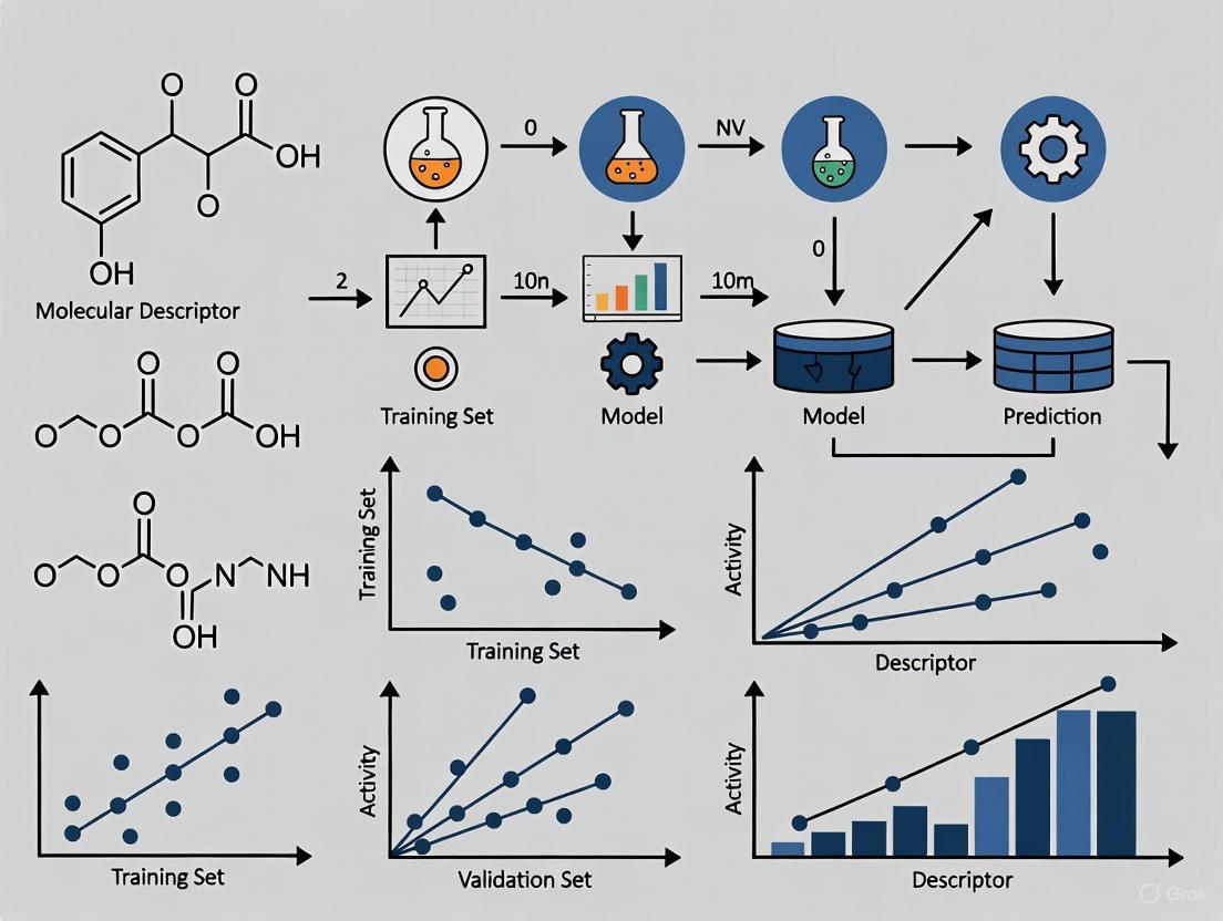
Figure 1: QSAR Modeling Workflow: The comprehensive process for developing and validating QSAR models, from data preparation through to application.

Data Preparation and Preprocessing

The foundation of any robust QSAR model is high-quality data. The initial stage involves compiling a dataset of chemical structures and their associated biological activities from reliable sources such as literature, patents, and experimental data [11]. Data curation must address several critical aspects: removal of duplicate or erroneous entries, standardization of chemical structures (including handling of salts, tautomers, and stereochemistry), and conversion of biological activities to consistent units [11]. Appropriate data splitting into training, validation, and external test sets is essential for proper model development and evaluation [11].

Feature Selection and Model Building

With numerous molecular descriptors typically available, feature selection becomes crucial to identify the most relevant descriptors and avoid overfitting [11]. Common feature selection methods include filter methods (ranking descriptors based on individual correlation), wrapper methods (using the modeling algorithm to evaluate descriptor subsets), and embedded methods (feature selection as part of model training) [11].

The choice of modeling algorithm depends on the complexity of the structure-activity relationship and the available data. Classical approaches include Multiple Linear Regression (MLR) and Partial Least Squares (PLS), while machine learning methods encompass Support Vector Machines (SVM), Random Forests (RF), and Neural Networks (NN) [11] [13].

Table 3: QSAR Modeling Algorithms and Their Applications

Algorithm	Type	Key Features	Best Suited For
Multiple Linear Regression (MLR)	Linear	Simple, interpretable, assumes linear relationship [11] [10]	Congeneric series with clear linear structure-activity relationships
Partial Least Squares (PLS)	Linear	Handles multicollinearity, works with many descriptors [14] [11]	3D-QSAR (CoMFA, CoMSIA), datasets with correlated descriptors
Support Vector Machines (SVM)	Non-linear	Captures complex relationships, robust to overfitting [11] [15]	Non-linear relationships, smaller datasets with complex patterns
Random Forests (RF)	Non-linear	Handles noisy data, built-in feature selection [15] [13]	Large, complex datasets, robust predictive modeling
Neural Networks (NN)	Non-linear	Flexible, learns intricate patterns, deep learning architectures [16] [13]	Very large datasets, complex non-linear relationships, deep learning applications

Model Validation and Applicability Domain

Rigorous validation is essential to ensure the reliability and predictive power of QSAR models. Validation assesses both the internal robustness of the model and its external predictivity for new compounds [2].

Validation Techniques

Internal validation employs the training data to estimate model performance, typically through cross-validation techniques. Leave-one-out (LOO) cross-validation involves using a single compound as the test set and the remainder as training, repeating this process for all compounds [11] [10]. k-fold cross-validation divides the training set into k subsets, using k-1 for training and one for testing, rotating through all subsets [11].

External validation uses an independent test set that was not involved in model development, providing a more realistic assessment of predictive performance on unseen data [11] [2]. Additional validation methods include data randomization (Y-scrambling) to verify the absence of chance correlations, and assessment of the model's applicability domain (AD) to define the chemical space where reliable predictions can be made [2].

Figure 2: QSAR Validation Framework: Comprehensive strategy for assessing model robustness, predictivity, and applicability domain.

Validation Metrics

Key metrics for evaluating QSAR models include R² (coefficient of determination) for goodness of fit, Q² (cross-validated R²) for internal predictive ability, and root mean square error (RMSE) for prediction errors [16] [2]. For classification QSAR models, additional metrics such as accuracy, sensitivity, specificity, and receiver operating characteristic (ROC) curves are employed [15].

Advanced QSAR Approaches in Machine Learning Research

The integration of machine learning with QSAR modeling has significantly expanded capabilities for drug discovery and chemical property prediction. Contemporary approaches leverage advanced algorithms and novel molecular representations to capture complex structure-activity relationships.

Machine Learning-Enhanced QSAR

Machine learning algorithms have dramatically improved QSAR predictive power, particularly for handling complex, high-dimensional chemical datasets [13]. Random Forests are valued for their robustness, built-in feature selection, and ability to handle noisy data, while Support Vector Machines excel in scenarios with limited samples and high descriptor-to-sample ratios [13]. Recent advances focus on improving model interpretability through techniques such as SHAP (SHapley Additive exPlanations) and LIME (Local Interpretable Model-agnostic Explanations), which help identify which descriptors most influence predictions [13].

Deep Learning and Graph-Based Approaches

Deep learning architectures have enabled the development of learned molecular representations without manual descriptor engineering [13]. Graph Neural Networks (GNNs) operate directly on molecular graphs, treating atoms as nodes and bonds as edges, thereby capturing inherent structural information [13]. SMILES-based transformers apply natural language processing techniques to chemical structures represented as text strings, allowing the model to learn complex patterns from large chemical databases [13].

3D-QSAR and Structural Methods

3D-QSAR approaches incorporate spatial molecular properties, providing enhanced capability for modeling steric and electrostatic interactions. Comparative Molecular Field Analysis (CoMFA) and Comparative Molecular Similarity Index Analysis (CoMSIA) represent prominent 3D-QSAR techniques that sample steric and electrostatic fields around aligned molecules [14]. These methods typically employ Partial Least Squares (PLS) regression for model building due to the high dimensionality of the field descriptors [14]. Recent advancements integrate machine learning with 3D-QSAR, demonstrating superior performance compared to traditional methods [15].

Experimental Protocols and Research Toolkit

Standard QSAR Development Protocol

A typical QSAR development protocol involves the following detailed steps:

• Dataset Compilation: Collect a minimum of 20-30 compounds with consistent biological activity data from a common experimental protocol to ensure comparable potency values [10]. The dataset should cover a diverse but relevant chemical space to the problem domain [11].

• Structure Standardization: Remove salts, normalize tautomers, handle stereochemistry consistently, and generate canonical representations using tools such as RDKit or OpenBabel [11].

• Descriptor Calculation: Compute molecular descriptors using software such as DRAGON, PaDEL-Descriptor, or Mordred [11]. Include diverse descriptor types (constitutional, topological, electronic, geometric) to comprehensively represent molecular features.

• Data Preprocessing: Address missing values through removal or imputation methods. Scale descriptors to zero mean and unit variance to ensure equal contribution during model training [11]. Split data into training (~70-80%), validation (~10-15%), and external test sets (~10-15%) using algorithms such as Kennard-Stone to ensure representative sampling [11].

• Feature Selection: Apply appropriate feature selection methods (filter, wrapper, or embedded) to identify the most relevant descriptors and reduce overfitting [11]. Ensure selected descriptors are not highly correlated to avoid multicollinearity issues [10].

• Model Training: Build models using selected algorithms, optimizing hyperparameters through grid search or Bayesian optimization with cross-validation [13]. For neural networks, optimize architecture, learning rate, and regularization parameters.

• Model Validation: Perform internal validation through cross-validation, external validation using the test set, and robustness checks through Y-scrambling [11] [2]. Define the applicability domain to identify where the model can make reliable predictions [2].

The QSAR Researcher's Toolkit

Table 4: Essential Resources for QSAR Modeling

Resource Category	Specific Tools/Software	Primary Function	Key Features
Descriptor Calculation	DRAGON, PaDEL-Descriptor, RDKit, Mordred [11] [13]	Generation of molecular descriptors	Comprehensive descriptor libraries, batch processing capabilities
Chemical Structure Handling	RDKit, OpenBabel, ChemAxon [11]	Structure standardization, format conversion	SMILES parsing, tautomer normalization, stereochemistry handling
Machine Learning Libraries	scikit-learn, TensorFlow, PyTorch [13]	Implementation of ML algorithms	Pre-built algorithms, neural network architectures, visualization tools
Specialized QSAR Software	SYBYL (CoMFA, CoMSIA), QSARINS, Build QSAR [14] [13]	Dedicated QSAR model development	3D-QSAR capabilities, model validation workflows, visualization
Molecular Docking	MOE, Schrödinger Suite, GOLD, AutoDock [14]	Structure-based drug design	Protein-ligand docking, binding pose prediction, scoring functions
Data Sources	ChEMBL, PubChem, Food Animal Residue Avoidance Databank [16]	Experimental biological activity data	Large compound databases, curated bioactivity data, ADMET properties

The fundamental equation of QSAR represents the mathematical embodiment of the structure-activity principle that has guided drug discovery and chemical design for decades. As QSAR methodologies have evolved from classical statistical approaches to contemporary machine learning and deep learning frameworks, the core objective remains unchanged: to establish quantitative, predictive relationships between molecular structure and biological activity.

The integration of artificial intelligence with QSAR modeling has created powerful synergies that enhance predictive accuracy, enable processing of complex chemical spaces, and accelerate therapeutic discovery. These advancements are particularly relevant in the context of modern drug discovery challenges, where the ability to rapidly identify and optimize lead compounds provides significant strategic advantages. As QSAR methodologies continue to evolve, they will undoubtedly remain essential components of the computational chemist's toolkit, bridging the gap between molecular structure and biological function through quantitative, data-driven approaches.

In modern Quantitative Structure-Activity Relationship (QSAR) modeling, molecular descriptors serve as the fundamental language that translates chemical structures into numerical data amenable to machine learning analysis. These quantitative representations of molecular properties provide the input features that enable artificial intelligence (AI) algorithms to establish mathematical relationships between chemical structure and biological activity [3] [17]. The evolution of QSAR from classical statistical methods to advanced machine learning frameworks has further elevated the importance of well-chosen molecular descriptors, as they directly influence model accuracy, interpretability, and predictive power [3].

Molecular descriptors encompass a wide spectrum of chemical information, ranging from simple atom counts to complex quantum-chemical properties and three-dimensional structural parameters [17]. The strategic selection and engineering of these descriptors is crucial for building robust QSAR models that can effectively navigate chemical space and generate reliable predictions for drug discovery applications [3] [18]. This technical guide examines the core categories of molecular descriptors essential for contemporary QSAR research, with particular emphasis on their computational derivation, strategic application in machine learning pipelines, and significance for rational drug design.

Molecular Descriptor Fundamentals

Definition and Purpose in QSAR

Molecular descriptors are numerical representations that encode chemical information derived from a molecule's structure [11] [17]. In QSAR modeling, they function as independent variables (features) that correlate with a dependent biological activity or property, forming the basis for predictive model building [11]. The underlying principle is that structural variations systematically influence biological activity, and these relationships can be captured mathematically through appropriate descriptor-activity mappings [11].

The calculation of molecular descriptors typically occurs after chemical structure standardization, which may include removal of salts, normalization of tautomers, and handling of stereochemistry [11]. Subsequently, specialized software tools generate hundreds to thousands of descriptor values for each compound, creating the feature matrix used for model training and validation [11] [17].

Integration with Machine Learning Workflows

In AI-driven QSAR, molecular descriptors serve as critical inputs for various machine learning algorithms, from traditional methods like Partial Least Squares (PLS) to advanced techniques including Random Forests, Support Vector Machines (SVM), and Graph Neural Networks (GNNs) [3] [11]. The choice and quality of descriptors significantly impact model performance, with optimal feature selection helping to mitigate overfitting and enhance interpretability [3] [18].

Recent innovations include "deep descriptors" learned automatically by neural networks from molecular graphs or SMILES strings, which can capture hierarchical chemical features without manual engineering [3]. However, traditional knowledge-driven descriptors remain vital for model interpretability and providing medicinal chemists with actionable insights for compound optimization [3] [17].

Table 1: Categories of Molecular Descriptors in QSAR Modeling

Category	Description	Examples	QSAR Applications
Constitutional	Simple counts of atoms, bonds, and functional groups	Molecular weight, number of H-bond donors/acceptors, rotatable bonds	Preliminary screening, drug-likeness filters (e.g., Lipinski's Rule of 5)
Topological	Based on molecular connectivity and graph theory	Topological indices, molecular connectivity indices, Kier-Hall indices	Modeling absorption, permeability, and basic pharmacophore patterns
Electronic	Describe electronic distribution and properties	HOMO/LUMO energies, dipole moment, molecular orbital energies	Predicting reactivity, metabolism, and target interaction mechanisms
3D Descriptors	Derived from three-dimensional molecular structure	Molecular surface area, volume, polar surface area, shape indices	Protein-ligand docking, binding affinity prediction, complex activity relationships
4D Descriptors	Account for conformational flexibility and ensembles	Conformer-dependent properties, interaction energy fields	Enhanced prediction accuracy for flexible molecules with multiple bioactive conformations

Constitutional Descriptors

Definition and Calculation

Constitutional descriptors represent the most fundamental category of molecular descriptors, consisting of simple counts of atoms, bonds, and functional groups within a molecule [11] [17]. These zero-dimensional descriptors are calculated directly from the molecular formula or connection table without considering atomic connectivity or spatial arrangement. Common examples include molecular weight, counts of specific atom types (e.g., carbon, oxygen, nitrogen), number of rotatable bonds, hydrogen bond donors and acceptors, and ring counts [17].

The computation of constitutional descriptors is computationally inexpensive and deterministic, requiring only 2D molecular structure information. Tools like RDKit, PaDEL-Descriptor, and Dragon can rapidly generate these descriptors for large compound libraries [11] [17].

Applications in Drug Discovery

Constitutional descriptors form the basis for drug-likeness filters such as Lipinski's Rule of Five, which uses molecular weight, H-bond donors, H-bond acceptors, and calculated logP to identify compounds with likely poor oral bioavailability [17]. In QSAR modeling, these descriptors provide baseline chemical information that often correlates with fundamental physicochemical properties and ADMET (Absorption, Distribution, Metabolism, Excretion, Toxicity) characteristics [18].

Despite their simplicity, constitutional descriptors frequently contribute significantly to QSAR models for properties dominated by bulk molecular features. For instance, molecular weight and rotatable bond count are important predictors of membrane permeability and oral bioavailability [17]. However, their limited chemical specificity makes them insufficient alone for modeling complex structure-activity relationships, necessitating supplementation with more sophisticated descriptor types.

Topological Descriptors

Theoretical Foundation

Topological descriptors, also known as 2D descriptors, are derived from the graph representation of a molecule, where atoms correspond to vertices and bonds to edges [11] [17]. These descriptors encode patterns of molecular connectivity using mathematical approaches from graph theory, capturing structural characteristics such as branching, cyclicity, and molecular complexity without requiring 3D coordinate information [17].

Key topological descriptors include various connectivity indices (e.g., Kier-Hall indices), path counts between atoms, and information-theoretic measures based on molecular symmetry and complexity [17]. These descriptors are typically generated from the hydrogen-suppressed molecular graph, focusing on the heavy atom skeleton and its connectivity pattern.

QSAR Applications and Significance

Topological descriptors have demonstrated exceptional utility in QSAR modeling across diverse applications. A comprehensive comparison of descriptor types for ADME-Tox prediction found that 2D descriptors frequently outperform fingerprint-based representations for targets including Ames mutagenicity, hERG inhibition, and blood-brain barrier permeability [18]. The study revealed that models built using traditional 2D descriptors achieved superior performance compared to those using Morgan fingerprints or MACCS keys across multiple machine learning algorithms [18].

The strength of topological descriptors lies in their ability to capture molecular complexity and substructural patterns that correlate with biological activity while remaining invariant to molecular conformation and orientation [17]. This makes them particularly valuable for high-throughput screening applications where 3D structure information may be unavailable or computationally prohibitive. Additionally, certain topological descriptors offer favorable interpretability, allowing medicinal chemists to trace model predictions back to specific structural features for rational drug design [11].

Electronic Descriptors

Quantum Chemical Foundations

Electronic descriptors quantify the electronic distribution and reactivity properties of molecules, derived from quantum mechanical calculations that solve the electronic Schrödinger equation for molecular systems [3] [17]. These descriptors provide insight into how molecules interact with biological targets through electrostatic, polar, and charge-transfer interactions. Essential electronic descriptors include HOMO-LUMO energies (Highest Occupied and Lowest Unoccupied Molecular Orbitals), HOMO-LUMO gap, dipole moment, atomic partial charges, and electrostatic potential surfaces [3] [17].

The computation of electronic descriptors typically involves quantum chemistry methods such as Density Functional Theory (DFT), which offers an optimal balance between accuracy and computational cost for drug-sized molecules [3]. Recent advances include machine learning potentials that dramatically accelerate these calculations while maintaining quantum-level accuracy [19].

Applications in Mechanism-Based QSAR

Electronic descriptors are indispensable for modeling biological activities where electronic interactions dominate the structure-activity relationship. The HOMO-LUMO gap, representing the energy required for electron excitation, frequently correlates with metabolic stability and reactivity [3]. Dipole moments and electrostatic potential maps help predict binding orientations in protein active sites and solvation effects [17].

In studies of persistent organic pollutants (POPs), HOMOEnergyDMol3 emerged as a critical descriptor for predicting air half-lives, reflecting the importance of electron donation capability in atmospheric degradation processes [20]. For drug discovery applications, electronic descriptors enhance predictions of metabolic transformations, toxicity mechanisms, and targeted protein degradation systems like PROTACs, where electronic properties influence the formation of ternary complexes [3].

3D Molecular Descriptors

Structural and Conformational Representation

3D molecular descriptors encode information derived from the three-dimensional structure of molecules, including spatial arrangement, shape, and surface properties [3] [17]. These descriptors require generation of low-energy conformations, typically through molecular mechanics force fields or quantum chemical optimization [17]. Common 3D descriptors include molecular surface area (van der Waals, solvent-accessible), molecular volume, polar surface area (PSA), radius of gyration, and principal moments of inertia [17].

Advanced 3D descriptors capture more complex spatial properties, such as Comparative Molecular Field Analysis (CoMFA) fields that represent steric and electrostatic interactions at grid points around the molecule, and shape descriptors that quantify molecular similarity based on volume overlap [3]. The generation of these descriptors necessitates careful conformational analysis to identify representative structures, often focusing on the presumed bioactive conformation [17].

Applications in Structure-Based Drug Design

3D descriptors excel in QSAR applications where molecular shape and spatial complementarity to biological targets significantly influence activity. They are particularly valuable for structure-based drug design, enabling correlation of structural features with binding affinity when protein structure information is available [3]. Polar Surface Area (PSA) has become a widely adopted descriptor for predicting membrane permeability, including blood-brain barrier penetration [17] [18].

The evolution beyond 3D to 4D descriptors incorporates conformational flexibility by considering ensembles of molecular structures rather than single static conformations [3]. These ensemble-based descriptors provide more realistic representations of molecules under physiological conditions and have demonstrated improved performance in QSAR refinement and ligand-based pharmacophore modeling [3]. Recent studies indicate that while 3D descriptors can enhance model accuracy for specific endpoints, their performance advantage over comprehensive 2D descriptors is often target-dependent [18].

Table 2: Computational Tools for Molecular Descriptor Calculation

Software Tool	Descriptor Coverage	Key Features	License
RDKit	Comprehensive 1D, 2D, limited 3D	Open-source, Python integration, descriptor importance analysis	Open-source
PaDEL-Descriptor	1D, 2D, and fingerprint types	Standalone software, 2D only, fast calculation of ~1875 descriptors	Free
Dragon	Extensive (over 5,000 descriptors)	Commercial grade, broad descriptor range, well-validated	Commercial
Mordred	1D, 2D (over 1,800 descriptors)	Python-based, compatible with scikit-learn	Open-source
Schrödinger	Comprehensive 2D, 3D, quantum	Integrated drug discovery suite, high-quality 3D structures	Commercial

Experimental Protocols for Descriptor Evaluation

Benchmarking Methodology for Descriptor Performance

Rigorous evaluation of molecular descriptor sets requires systematic benchmarking protocols. A representative methodology involves curating diverse datasets with known biological activities, calculating multiple descriptor types, and building QSAR models using different machine learning algorithms with standardized validation procedures [18]. For example, in ADME-Tox descriptor comparisons, datasets should include 1,000+ compounds with balanced active/inactive ratios for reliable statistics [18].

The experimental workflow typically includes: (1) data curation (removing duplicates, standardizing structures, handling missing values); (2) descriptor calculation using multiple software tools; (3) descriptor preprocessing (removing constant and highly correlated variables, normalization); (4) model building with various algorithms (e.g., XGBoost, SVM, Neural Networks); and (5) comprehensive validation using both internal (cross-validation) and external test sets [11] [18]. Performance metrics should extend beyond simple accuracy to include area under ROC curve, precision-recall curves, and applicability domain assessment [11] [18].

Case Study: ADME-Tox Descriptor Comparison

A recent benchmark study compared descriptor performance across six ADME-Tox targets (Ames mutagenicity, P-glycoprotein inhibition, hERG inhibition, hepatotoxicity, blood-brain barrier permeability, and CYP 2C9 inhibition) using two machine learning algorithms (XGBoost and RPropMLP) [18]. The research implemented strict data curation protocols including salt removal, element filtering (C, H, N, O, S, P, F, Cl, Br, I), and 3D structure optimization with Schrödinger's Macromodel [18].

Results demonstrated that traditional 2D descriptors frequently outperformed fingerprint-based representations, with 2D descriptors producing superior models for almost every dataset compared to descriptor combinations [18]. This finding highlights the enduring value of well-curated 2D descriptors despite the increasing popularity of fingerprint-based approaches and deep learning representations.

Visualization of QSAR Workflow with Molecular Descriptors

This workflow diagram illustrates the systematic process of incorporating diverse molecular descriptors into QSAR modeling pipelines, highlighting how different descriptor categories contribute to machine learning-based activity prediction and drug design.

Table 3: Essential Computational Tools for Descriptor-Based QSAR

Tool/Resource	Type	Primary Function	Application in QSAR
RDKit	Cheminformatics Library	Molecular descriptor calculation and fingerprint generation	Open-source platform for calculating 1D, 2D descriptors and molecular fingerprints [17]
PaDEL-Descriptor	Software Package	Molecular descriptor and fingerprint calculation	Standalone tool for calculating ~1875 molecular descriptors and 12 types of fingerprints [11] [17]
Dragon	Commercial Software	Comprehensive descriptor calculation	Industry-standard tool generating >5,000 molecular descriptors for QSAR modeling [3] [17]
Schrödinger Suite	Commercial Drug Discovery Platform	Molecular modeling and descriptor calculation	Integrated environment for generating high-quality 3D structures and advanced molecular descriptors [18]
scikit-learn	Machine Learning Library	Model building and feature selection	Python library for machine learning algorithms, feature selection, and model validation in QSAR [3]
AutoDock/Gnina	Molecular Docking Software	Protein-ligand docking and pose prediction	Structure-based approaches that complement ligand-based QSAR; Gnina uses CNN for scoring poses [19]

Emerging Trends and Future Directions

The field of molecular descriptors continues to evolve with several emerging trends shaping future QSAR research. Causal inference frameworks are being developed to address confounding in high-dimensional descriptor spaces, using methods like Double Machine Learning to identify descriptors with genuine causal effects on biological activity rather than mere correlation [21]. Quantum machine learning approaches demonstrate potential advantages for QSAR prediction, particularly when dealing with limited data availability, as quantum classifiers may offer superior generalization power with reduced feature sets [22].

The integration of AI-generated descriptors with traditional knowledge-based representations represents a promising direction, combining the pattern recognition strength of deep learning with the interpretability of established descriptors [3] [19]. Additionally, federated learning approaches enable collaborative model development across institutions while preserving data privacy, facilitating the creation of more robust QSAR models using diverse chemical datasets without sharing proprietary information [23].

As these advancements mature, molecular descriptors will continue to serve as the foundational elements connecting chemical structure to biological activity, driving innovation in drug discovery through increasingly sophisticated QSAR methodologies that leverage the complementary strengths of computational chemistry and machine learning.

In the contemporary landscape of drug discovery and environmental chemistry, Quantitative Structure-Activity Relationship (QSAR) modeling has emerged as a pivotal computational approach that mathematically links a chemical compound's structure to its biological activity or physicochemical properties [11]. The foundation of any robust QSAR model rests on three critical pillars: a high-quality dataset of molecules with known activities, powerful machine learning algorithms to discern complex patterns, and sophisticated software tools that can translate molecular structures into numerical representations known as descriptors [24]. These molecular descriptors quantitatively capture structural, physicochemical, and electronic properties of molecules, serving as the essential input variables for QSAR models [11] [25].

The evolution of cheminformatics platforms has fundamentally transformed QSAR research from a traditionally linear, hypothesis-driven discipline to a data-rich, artificial intelligence (AI)-powered paradigm [24]. Modern QSAR workflows now leverage advanced machine learning (ML) and deep learning techniques to navigate complex chemical spaces and predict biological activities with remarkable accuracy. This whitepaper provides a comprehensive technical overview of essential software tools—including open-source solutions like PaDEL, RDKit, and Dragon, alongside leading commercial platforms—that are shaping the future of QSAR research in 2025. By examining their capabilities, integration potential, and specific applications in ML-driven QSAR workflows, this guide aims to equip researchers, scientists, and drug development professionals with the knowledge to select and implement the most appropriate tools for their computational research objectives.

Core Open-Source Cheminformatics Tools

Open-source cheminformatics tools have become fundamental components of modern QSAR research pipelines, offering transparency, flexibility, and cost-effectiveness. These tools primarily function as molecular descriptor calculators and chemical intelligence engines that feed machine learning algorithms with structurally encoded information.

RDKit: The Open-Source Standard

RDKit is an open-source cheminformatics toolkit (BSD-licensed) written in C++ with Python bindings that has become a de facto standard in the field due to its comprehensive functionality, high performance, and active community [26]. While RDKit is a library rather than a standalone graphical application, it provides robust core chemistry functions including molecule I/O, substructure search, fingerprint generation, descriptor calculation, and chemical reaction handling [26]. Its continuous development and updating by the community ensures it remains at the forefront of cheminformatics methodology.

RDKit offers a rich set of molecular fingerprint algorithms and similarity functions, including Morgan fingerprints (circular fingerprints akin to ECFP), classical Daylight-type path fingerprints (RDKit Fingerprint), Topological Torsion and Atom Pair fingerprints, and MACCS keys [26]. These fingerprints serve as critical inputs for machine learning models, particularly for similarity searching and clustering tasks. The toolkit also provides extensive capabilities for virtual screening through fast substructure searches and 2D similarity searches on large chemical libraries, especially when combined with its PostgreSQL cartridge or in-memory fingerprint indices [26]. A key strength of RDKit lies in its integration potential; it features Python, C++, Java, and JavaScript interfaces, allowing it to plug into diverse environments and connect with docking programs, machine learning frameworks, and visualization tools [26].

Dragon and E-Dragon: The Descriptor Specialists

Dragon is a specialized application for calculating molecular descriptors, developed by the Milano Chemometrics and QSAR Research Group [25]. It represents one of the most comprehensive descriptor calculation tools available, generating more than 1,600 molecular descriptors divided into 20 logical blocks [25]. These descriptors encompass everything from simple atom type and functional group counts to complex topological, geometrical, and constitutional descriptors [25]. Dragon requires 3D optimized molecular structures with hydrogen atoms as input, accepting common molecular file formats [25].

The E-Dragon platform provides a web-accessible interface to Dragon's descriptor calculation capabilities, though with some limitations—it can analyze a maximum of 149 molecules and 150 atoms per molecule using the Dragon 5.4 version [25]. For researchers requiring 3D structure generation, E-Dragon integrates CORINA (provided by Molecular Networks GMBH) to calculate 3D atom coordinates when unavailable in the input files [25]. Dragon's extensive descriptor sets have been widely adopted in regulatory and research applications, forming the computational foundation for numerous QSAR projects and models, including those integrated into the US EPA's Toxicity Estimation Software Tool (TEST) and the European CAESAR project for REACH legislation implementation [27].

PaDEL-Descriptor: The Java-Based Alternative

PaDEL-Descriptor is an open-source alternative for molecular descriptor calculation, designed as a Java-based application that provides a comprehensive suite of descriptor and fingerprint calculation capabilities [11]. While the search results provide limited specific details about PaDEL-Descriptor, it is recognized alongside Dragon, RDKit, Mordred, ChemAxon, and OpenBabel as one of the primary software packages available to calculate a wide variety of molecular descriptors [11]. These tools can generate hundreds to thousands of descriptors for a given set of molecules, making careful selection of the most relevant descriptors crucial for building robust and interpretable QSAR models [11].

Table 1: Comparison of Core Open-Source Cheminformatics Tools

Tool	Primary Function	Descriptor Count	Key Features	Input Requirements	Integration & Licensing
RDKit	Comprehensive cheminformatics	Not specified (wide variety)	Multiple fingerprint types, substructure search, 3D conformer generation, Python/C++ APIs	SMILES, SDF, Mol, etc.	Open-source (BSD), Python/C++/Java/JS bindings, KNIME nodes
Dragon	Molecular descriptor calculation	>1,600 descriptors [25]	20 descriptor blocks, extensive topological/geometrical descriptors	3D optimized structures with hydrogens	Commercial, used in TEST, CAESAR, OCHEM [27]
E-Dragon	Online descriptor calculation	>1,600 descriptors [25]	Web-based Dragon interface, integrated 3D structure generation	SMILES, SDF, MOL2 files	Free web service (149 molecule limit) [25]
PaDEL-Descriptor	Descriptor & fingerprint calculation	Not specified (comprehensive)	Java-based, cross-platform compatibility	Molecular structure files	Open-source [11]

Commercial Cheminformatics Platforms

Commercial cheminformatics platforms offer integrated, user-friendly solutions that often combine descriptor calculation, model building, and visualization capabilities within unified environments. These platforms are particularly valuable in regulated industries and for organizations requiring robust technical support.

MOE (Molecular Operating Environment)

The Chemical Computing Group's MOE offers an all-in-one platform for drug discovery that integrates molecular modeling, cheminformatics, and bioinformatics [28]. MOE excels in structure-based drug design, molecular docking, and QSAR modeling, while supporting critical tasks like ADMET prediction and protein engineering [28]. Its user-friendly interface and interactive 3D visualization tools make it accessible for a wide range of researchers, from computational specialists to medicinal chemists. MOE employs modular workflows, machine learning integration, and flexible licensing options, positioning it as a comprehensive solution for organizations of all sizes [28].

Schrödinger Suite

Schrödinger's platform integrates advanced quantum chemical methods with machine learning approaches for molecular catalyst design and drug discovery [28]. Their flagship product, Live Design, provides an entry point into most of Schrödinger's tools with scalable licensing. A key differentiator is Schrödinger's development of novel scoring functions, including GlideScore, which is specifically designed to maximize separation of compounds with strong binding affinity from those with little to no binding ability [28]. The platform also includes DeepAutoQSAR, a machine learning solution for predicting molecular properties based on chemical structure [28]. Schrödinger has partnered with Google Cloud to substantially increase the speed and capacity of its physics-based molecule modeling platform, enabling the simulation of billions of potential compounds per week [28].

ChemAxon Suite

ChemAxon offers a comprehensive suite of cheminformatics software tools, including the Plexus Suite and Design Hub, which are widely used in industry for enterprise-level chemical data management [28] [26]. The Plexus Suite is a web-based software package that incorporates ChemAxon's chemistry capabilities for accessing, displaying, searching, and analyzing scientific data [28]. It includes specialized tools such as Plexus Connect for data querying and visualization, Plexus Design for virtual library design, and Plexus Mining for chemically intelligent data mining [28]. Design Hub serves as ChemAxon's platform for compound design and tracking in drug discovery, connecting scientific hypotheses, candidate compound selection, and computational capabilities [28].

OECD QSAR Toolbox

The OECD QSAR Toolbox represents a specialized category of regulatory-focused software, developed to promote the use of (Q)SAR technology in regulatory contexts by making it "readily accessible, transparent, and less demanding in terms of infrastructure costs" [29]. This software application is intended for use by governments, chemical industry, and other stakeholders in filling gaps in (eco)toxicity data needed for assessing the hazards of chemicals [29]. The Toolbox incorporates information and tools from various sources into a logical workflow, with chemical categorization forming a crucial component of its methodology [29]. Its development has occurred in multiple phases, with version 4.7 released in July 2024 and version 4.8 in July 2025 [29].

Table 2: Commercial Cheminformatics Platforms for QSAR Research

Platform	Primary Focus	Key QSAR Features	Target Users	Licensing Model
MOE	Integrated drug discovery	QSAR modeling, molecular docking, ADMET prediction, machine learning integration	Pharmaceutical R&D, academic research	Modular, flexible licensing [28]
Schrödinger	Physics-based modeling & ML	DeepAutoQSAR, quantum chemical methods, free energy calculations	Drug discovery organizations, computational chemists	Modular, scalable licensing [28]
ChemAxon	Chemical intelligence & enterprise data	Plexus Suite, Design Hub, chemical data management	Enterprise pharmaceutical companies, research institutions	Pay-per-use [28]
OECD QSAR Toolbox	Regulatory hazard assessment	Chemical categorization, read-across, (eco)toxicity prediction	Regulators, chemical industry, risk assessors	Free [29]
StarDrop	Small molecule design & optimization	Patented AI-guided optimization, QSAR models for ADME/physicochemical properties	Medicinal chemists, lead optimization teams	Modular pricing [28]
DataWarrior	Open-source data analysis & visualization	QSAR model development, molecular descriptors, machine learning integration	Academic researchers, small companies	Open-source [28]

Integrated Workflows: From Molecular Structures to QSAR Predictions

The true power of modern cheminformatics tools emerges when they are integrated into cohesive workflows that transform molecular structures into reliable QSAR predictions. This section outlines standardized protocols and methodologies for leveraging these tools in ML-driven QSAR research.

Standardized QSAR Modeling Workflow

A typical QSAR modeling workflow incorporates multiple steps from data compilation to model validation [11]. The process begins with dataset compilation of chemical structures and associated biological activities from reliable sources, ensuring the dataset is high-quality and representative of the chemical space of interest [11]. This is followed by data cleaning and preprocessing, which involves removing duplicates, standardizing chemical structures (e.g., removing salts, normalizing tautomers, handling stereochemistry), converting biological activities to common units, and handling outliers or missing values [11]. The next step involves molecular descriptor calculation using tools like Dragon, RDKit, or PaDEL-Descriptor to generate numerical representations of the structural, physicochemical, and electronic properties of the compounds [11].

Feature selection techniques are then applied to identify the most relevant descriptors, which helps avoid overfitting and improves model interpretability [11]. The curated dataset is subsequently split into training and test sets, often using methods like the Kennard-Stone algorithm, to enable proper model validation [11]. The core model building phase employs regression or classification algorithms such as multiple linear regression (MLR), partial least squares (PLS), random forest, or more advanced machine learning techniques [11]. Finally, the models undergo rigorous validation using internal (e.g., cross-validation) and external test sets to assess predictive performance and robustness, with careful evaluation of the applicability domain to determine the chemical space where the models can make reliable predictions [11].

Diagram 1: QSAR Modeling Workflow. This diagram illustrates the standardized workflow for QSAR model development, highlighting the integration points for various software tools at different stages.

Machine Learning Integration in QSAR

The integration of machine learning with cheminformatics tools has significantly expanded the capabilities of QSAR modeling. Modern QSAR research employs a diverse array of ML algorithms, ranging from traditional methods to advanced deep learning techniques [30]. Commonly used algorithms include Support Vector Machines (SVM), which are particularly effective for handling non-linear relationships in high-dimensional descriptor spaces; Random Forests, which provide robust performance and feature importance metrics; Artificial Neural Networks (ANNs), which can capture complex non-linear patterns; and Gradient Boosting methods, which often deliver state-of-the-art predictive performance [24].

The selection between linear and non-linear QSAR models depends on the complexity of the structure-activity relationship and the size and quality of the available data [11]. Linear models, including Multiple Linear Regression (MLR) and Partial Least Squares (PLS), assume a straightforward relationship between molecular descriptors and biological activity, offering higher interpretability but potentially limited predictive power for complex endpoints [11]. Non-linear models, including those based on ANN or SVM, can capture more intricate patterns but require larger datasets for training and are more prone to overfitting without proper validation [11]. A comparative study highlighted this distinction, demonstrating that while both linear PLS and non-linear ANN QSAR models were developed for predicting the antioxidant capacity of phenolic compounds, the non-linear ANN model showed stronger predictive performance, underscoring the importance of non-linear relationships between molecular descriptors and biological activity in many scenarios [11].

Advanced Applications: Case Study on Cyclodextrin Complexes

Recent advances in QSAR methodologies are exemplified by sophisticated applications such as predicting the thermodynamic stability of cyclodextrin inclusion complexes [24]. Cyclodextrins are macrocyclic rings composed of glucose residues that form host-guest inclusion complexes, making them valuable in pharmaceutical, cosmetic, and food industries [24]. QSAR/QSPR approaches have been successfully employed to predict stability constants (log K) for these complexes, utilizing molecular descriptors of guest molecules in conjunction with various machine learning algorithms [24].

This application demonstrates the power of integrating comprehensive descriptor sets (such as those generated by Dragon or RDKit) with advanced ML techniques to address complex molecular interaction problems. The success of these models relies on three crucial components: a high-quality dataset of experimental stability constants, comprehensive molecular descriptors characterizing guest structure and physicochemistry, and appropriate ML algorithms that quantitatively express the relationship between descriptors and complex stability [24]. Such advanced applications highlight the growing sophistication of QSAR methodologies and their utility in predicting complex molecular interactions beyond traditional biological activity endpoints.

Essential Research Reagents and Computational Solutions

The experimental and computational infrastructure supporting modern QSAR research comprises both software tools and critical data resources. The table below details key "research reagent solutions" essential for conducting robust QSAR studies.

Table 3: Essential Research Reagents & Computational Solutions for QSAR Research

Resource Category	Specific Tools/Databases	Function in QSAR Research	Access & Licensing
Descriptor Calculation Tools	Dragon, RDKit, PaDEL-Descriptor, Mordred	Generate numerical representations of molecular structures for ML model input	Commercial, Open-source [11]
Integrated Modeling Platforms	MOE, Schrödinger, StarDrop, OECD QSAR Toolbox	Provide end-to-end environments for QSAR model building and validation	Commercial, Free [28] [29]
Chemical Databases	PubChem, DrugBank, ZINC15, ChEMBL	Supply chemical structures and associated bioactivity data for training sets	Publicly accessible [31]
Machine Learning Frameworks	Scikit-learn, TensorFlow, PyTorch, XGBoost	Implement algorithms for building predictive QSAR models	Open-source
Specialized QSAR Applications	CAESAR, TEST, OCHEM, VEGA	Offer pre-validated models for specific endpoints (toxicity, environmental fate)	Free, Web-based [32] [27]
Data Preprocessing Tools	RDKit, KNIME, Pipeline Pilot	Handle structure standardization, duplicate removal, feature scaling	Open-source, Commercial [11] [31]

The landscape of cheminformatics tools for QSAR research offers diverse solutions ranging from specialized open-source descriptor calculators to comprehensive commercial platforms. The strategic selection of appropriate tools depends on multiple factors, including research objectives, available computational expertise, regulatory requirements, and budget constraints. Open-source tools like RDKit and PaDEL-Descriptor provide unparalleled transparency and customization potential, making them ideal for academic research and method development. Commercial platforms such as MOE and Schrödinger offer integrated, user-friendly environments with robust technical support, catering well to industrial drug discovery pipelines. Regulatory-focused tools like the OECD QSAR Toolbox address specific needs for hazard assessment within regulatory frameworks.

As QSAR methodology continues to evolve, several trends are shaping tool development and application: the deepening integration of machine learning and artificial intelligence, the expansion of applicability domains to cover more complex endpoints, the growing importance of model interpretability and regulatory acceptance, and the emergence of hybrid approaches that combine multiple tools in optimized workflows. By understanding the capabilities, strengths, and limitations of the various software tools available, researchers can construct more effective, reliable, and predictive QSAR models that accelerate drug discovery, improve chemical safety assessment, and advance our fundamental understanding of structure-activity relationships across diverse chemical domains.

The Critical Importance of Data Curation and Standardization

In the realm of Quantitative Structure-Activity Relationship (QSAR) research, the pursuit of accurate, reliable, and universally applicable machine learning models is fundamentally dependent on the quality of the underlying data. QSAR modeling is a computational approach that mathematically links a chemical compound's structure to its biological activity or properties, playing a crucial role in drug discovery and environmental chemistry by prioritizing promising drug candidates and reducing animal testing [11]. These models operate on the principle that structural variations systematically influence biological activity, using physicochemical properties and molecular descriptors as predictor variables [11]. While advancements in mathematical algorithms and descriptor development have propelled the field forward, the generalization capability and predictive power of any QSAR model are ultimately constrained by the data from which it is derived [33]. As one comprehensive review notes, "a high-quality dataset is the cornerstone of building an effective QSAR model" [33]. Within a broader thesis on machine learning for QSAR, this whitepaper establishes why rigorous data curation and standardization are not merely preliminary steps but continuous, critical processes that determine the success or failure of computational predictive modeling in chemical sciences.

The development of QSAR models applicable to general molecules remains a significant challenge, primarily due to issues of molecular structure representation, inadequacy of molecular datasets, and limitations in model interpretability and predictive power [33]. These challenges underscore the necessity for meticulous data management. The "garbage in, garbage out" paradigm is particularly pertinent; without precise molecular descriptors and standardized, high-quality data, even the most sophisticated deep learning architectures will produce unreliable predictions [33]. This paper provides researchers, scientists, and drug development professionals with a technical examination of data curation methodologies, experimental protocols for data standardization, and practical visualization tools to enhance the reliability and regulatory acceptance of QSAR models in real-world applications.

The Critical Role of Data in QSAR Modeling

Fundamental Data Requirements for Robust QSAR

QSAR models are fundamentally data-driven, constructed based on molecular training sets that must satisfy several critical criteria to ensure model validity [33]. The quality and representativeness of these datasets directly influence a model's prediction and generalization capabilities [33]. Three primary data characteristics are essential:

• Structural Diversity: Datasets must encompass a wide variety of chemical structures to adequately represent the chemical space of interest, enabling models to recognize patterns beyond narrow structural classes [33] [11].
• Quantitative Activity Data: Biological activity data, typically obtained through rigorous experimentation, should be quantitative, consistently measured, and expressed in standardized units (e.g., Ki, IC50) to allow for meaningful comparative analysis [34] [11].
• Mechanistic Relevance: The structural features and descriptors encoded in the dataset should have plausible correlations with the biological activity or property being modeled, reflecting underlying mechanistic relationships [33].

Pursuing a universal QSAR model capable of reliably predicting the properties of general molecules poses significant data challenges. It requires "having a sufficient number of structure-activity relationship instances as training data to cope with the complexity and diversity of molecular structures and action mechanisms" [33]. This necessitates not only large volumes of data but also broad coverage of chemical space and biological endpoints.

Consequences of Inadequate Data Practices

Failure to implement robust data curation and standardization protocols leads to several critical failures in QSAR modeling:

• Poor Predictive Accuracy: Models trained on uncurated data often fail to generalize beyond their training set, producing inaccurate predictions for new chemical entities [33].
• Limited Applicability Domain: The chemical space where models can make reliable predictions becomes artificially constrained when datasets lack diversity or contain biases [33].
• Reduced Regulatory Acceptance: Regulatory agencies increasingly require transparent documentation of data quality and standardization procedures, with inadequate practices limiting the use of models in safety assessment [35].

The GenoITS workflow for genotoxicity assessment demonstrates the regulatory importance of standardized data, integrating experimental data and QSAR predictions within a structured framework following REACH regulations [35]. Such integration is only possible with rigorously curated and standardized data sources.

Data Curation: Methodologies and Protocols

Data curation encompasses the comprehensive process of collecting, cleaning, and preparing chemical and biological data for QSAR modeling. The following experimental protocols detail the key stages of this process.

Dataset Collection and Compilation

The initial phase involves gathering a comprehensive set of chemical structures and their associated biological activities from reliable sources.

• Protocol 3.1.1: Multi-Source Data Aggregation
  • Objective: Compile a structurally diverse dataset representing the relevant chemical space.
  • Materials: Public databases (e.g., PubChem, ChEMBL), proprietary corporate databases, peer-reviewed literature, and patent sources.
  • Procedure:
    • Identify relevant data sources for the target endpoint (e.g., genotoxicity [35], ALK tyrosine kinase inhibition [34]).
    • Extract chemical structures in standardized formats (SMILES, InChI).
    • Collect associated biological activity values, noting experimental conditions and measurement types (Ki, IC50, etc.).
    • Record all metadata, including data sources, experimental conditions, and assay protocols.
  • Quality Control: Document data provenance thoroughly to ensure traceability and reliability [11].

Data Cleaning and Standardization

This critical phase addresses inconsistencies and errors in raw data to create a unified, analysis-ready dataset.

• Protocol 3.2.1: Structural Standardization

  • Objective: Create a consistent representation of all molecular structures.
  • Materials: Cheminformatics toolkits (e.g., RDKit, OpenBabel).
  • Procedure:
    • Remove Salts and Solvents: Strip counterions and solvent molecules to isolate the primary structure of interest.
    • Normalize Tautomers: Standardize tautomeric forms to a consistent representation.
    • Handle Stereochemistry: Explicitly define stereocenters using appropriate descriptors; consider generating distinct entries for stereoisomers if configuration is unspecified but activity varies.
    • Standardize Representation: Apply consistent atom ordering, bond typing, and hydrogen representation.
  • Quality Control: Visually inspect a subset of structures before and after standardization to verify accuracy.

• Protocol 3.2.2: Activity Data Harmonization

  • Objective: Convert all biological activities to a consistent scale and unit.
  • Materials: Scripting environment (e.g., Python, R) for data transformation.
  • Procedure:
    • Convert all activity values to a common unit (e.g., nM for concentration-based measures).
    • Transform to a logarithmic scale (e.g., pKi = -log(Ki)) when appropriate to normalize the distribution for modeling.
    • Identify and document significant outliers for potential exclusion based on statistical criteria or evidence of experimental error.
  • Quality Control: Generate distribution plots of activity values before and after transformation to verify consistency.

Table 1: Common Data Cleaning Operations and Their Impact on QSAR Model Quality

Data Issue	Standardization Protocol	Impact of Neglect on Model
Tautomeric Forms	Normalize to predominant tautomer at physiological pH	Artificial inflation of chemical diversity; incorrect descriptor calculation
Unspecified Stereochemistry	Treat as racemic mixture or create separate entries	Introduction of noise in activity data; reduced predictive accuracy for chiral compounds
Mixed Activity Units	Convert to consistent unit (e.g., nM) and scale (e.g., pIC50)	Mathematical inconsistencies; invalid model coefficients and predictions
Salt Forms	Remove counterions; represent parent structure	Incorrect molecular representation; skewed physicochemical property calculations

Handling Missing Values and Data Imputation

Missing data presents a common challenge in QSAR datasets that requires systematic handling.

• Protocol 3.3.1: Missing Data Assessment and Imputation
  • Objective: Address missing values while minimizing introduction of bias.
  • Materials: Statistical software packages.
  • Procedure:
    • Quantify the extent and pattern of missing data for each variable.
    • For datasets with <5% missing values for a given descriptor, consider removal of compounds with missing values.
    • For larger gaps, employ appropriate imputation techniques:
      • Mean/Median Imputation: Replace missing values with the variable mean or median (suitable for normally distributed data).
      • K-Nearest Neighbors (KNN) Imputation: Impute missing values based on similar compounds in the dataset.
      • QSAR-Based Imputation: Build a predictive model for the missing descriptor using other available descriptors.
    • Document all imputation procedures for transparency.
  • Quality Control: Compare model performance with and without imputation to assess impact.

The following workflow diagram visualizes the comprehensive data curation process from initial collection to prepared dataset, incorporating the key protocols outlined above:

Data Standardization for QSAR Modeling

Standardization ensures that molecular representations and biological responses are consistent, comparable, and suitable for computational analysis.

Molecular Descriptor Calculation and Standardization

Molecular descriptors are mathematical representations of structural, physicochemical, and electronic properties that serve as the input variables for QSAR models [33] [11]. The selection of appropriate descriptors is crucial, as they must "comprehensively represent molecular properties, correlate with biological activity, be computationally feasible, have distinct chemical meanings, and be sensitive enough to capture subtle variations in molecular structure" [33].

• Protocol 4.1.1: Descriptor Calculation and Preprocessing
  • Objective: Generate a comprehensive set of molecular descriptors and prepare them for modeling.
  • Materials: Descriptor calculation software (PaDEL-Descriptor, Dragon, RDKit, Mordred) [11].
  • Procedure:
    • Calculate a diverse set of descriptors covering constitutional, topological, electronic, geometric, and thermodynamic properties [11].
    • Remove constant or near-constant descriptors with no meaningful variance.
    • Identify and address correlated descriptor pairs (e.g., |r| > 0.95) to reduce multicollinearity.
    • Apply scaling (e.g., standardization to z-scores: (x - μ)/σ) to ensure all descriptors contribute equally during model training [11].
  • Quality Control: Generate correlation matrices and variance plots to verify descriptor preprocessing.

Table 2: Categories of Molecular Descriptors and Their Applications in QSAR

Descriptor Category	Description	Example Descriptors	QSAR Application Context
Constitutional	Atom and bond counts; molecular weight	Molecular weight, number of rotatable bonds, hydrogen bond donors/acceptors	High-throughput screening; preliminary absorption, distribution, metabolism, excretion, and toxicity (ADMET) profiling
Topological	Molecular connectivity patterns	Molecular connectivity indices, Wiener index, Zagreb index	Modeling transport properties; predicting boiling points and solubility
Electronic	Charge distribution and orbital properties	Partial atomic charges, dipole moment, highest occupied molecular orbital (HOMO)/lowest unoccupied molecular orbital (LUMO) energies	Modeling ligand-receptor interactions; predicting chemical reactivity
Geometric	3D shape and size parameters	Principal moments of inertia, molecular volume, surface area	Protein-ligand docking studies; enzyme inhibitor design

Dataset Division and Applicability Domain

Proper dataset division defines the scope within which a QSAR model can make reliable predictions.

• Protocol 4.2.1: Strategic Dataset Division
  • Objective: Partition data into training, validation, and test sets to enable robust model development and evaluation.
  • Materials: Cheminformatics toolkit with sampling capabilities.
  • Procedure:
    • External Test Set: Reserve 20-30% of compounds exclusively for final model assessment, ensuring they remain completely independent of model tuning and selection [11].
    • Training Set: Use the remaining 70-80% for model building and parameter estimation.
    • Validation Set: Further split the training set via cross-validation for hyperparameter tuning.
    • Apply structured sampling methods (e.g., Kennard-Stone) to ensure all sets adequately cover the chemical space [11].
  • Quality Control: Verify that activity distributions and structural diversity are similar across all splits.

The following diagram illustrates the relationship between data curation, standardization processes, and the resulting model quality and applicability domain:

The Scientist's Toolkit: Essential Research Reagents and Software

Successful implementation of QSAR data curation and standardization protocols requires specific computational tools and resources. The following table details essential solutions for building robust QSAR workflows.

Table 3: Essential Research Reagent Solutions for QSAR Data Curation and Modeling

Tool Category	Specific Tools/Software	Primary Function in QSAR	Application Context
Descriptor Calculation	PaDEL-Descriptor, Dragon, RDKit, Mordred [11]	Generation of molecular descriptors from chemical structures	Converting structural information into numerical representations for modeling; comprehensive molecular profiling
Cheminformatics Platforms	RDKit, OpenBabel, ChemAxon [11]	Chemical structure standardization, format conversion, basic descriptor calculation	Data preprocessing workflows; handling diverse chemical file formats; structural normalization
Data Analysis & Modeling	Python/R with scikit-learn, specialized QSAR packages	Statistical analysis, machine learning, model building and validation	Developing and validating QSAR models; feature selection; performance evaluation
Integrated Testing Systems	GenoITS [35]	Regulatory-grade toxicity prediction within standardized workflows	Safety assessment following REACH regulations; integrated testing strategies for genotoxicity

The exponential growth of chemical data and computational power presents unprecedented opportunities for advancing QSAR research. However, as highlighted throughout this technical guide, these opportunities can only be fully realized through unwavering commitment to rigorous data curation and standardized protocols. The development of "larger and higher-quality data sets, more accurate molecular descriptors and deep learning methods" promises continuous improvement in the predictive ability, interpretability, and application domain of QSAR models [33]. By implementing the systematic methodologies outlined for data collection, cleaning, standardization, and validation, researchers can significantly enhance the reliability and regulatory acceptance of their QSAR models. In an era where computational toxicology and in silico drug discovery are increasingly central to chemical safety assessment and pharmaceutical development, exemplary data practices become not just a scientific best practice but an ethical imperative for reducing animal testing and accelerating the development of safer, more effective chemicals and therapeutics [35].

Building and Applying Robust QSAR Models: A Step-by-Step Workflow

Quantitative Structure-Activity Relationship (QSAR) modeling represents a computational methodology that correlates the chemical structure of compounds with their biological activity using mathematical and statistical approaches [36]. The fundamental principle underpinning QSAR is that variations in molecular structure produce corresponding changes in biological activity, which can be quantified and predicted using computational models [37]. In the contemporary drug discovery landscape, QSAR has become an indispensable tool that significantly reduces development costs and time by prioritizing candidate compounds for synthesis and experimental testing, thereby minimizing extensive and ethically concerning animal testing [36] [38]. The integration of machine learning (ML) and artificial intelligence (AI) has further revolutionized QSAR modeling, enabling researchers to build more accurate and reliable predictive models that can navigate the complex chemical space of potential drug molecules [5] [38].

The evolution of QSAR methodologies has progressed from one-dimensional approaches correlating simple physicochemical parameters like pKa and logP to sophisticated multi-dimensional models that incorporate two-dimensional structural patterns, three-dimensional molecular conformations, and even higher-dimensional representations that account for ligand flexibility and multiple conformational states [36]. This technical guide provides a comprehensive examination of the complete QSAR modeling pipeline, framed within the broader context of machine learning applications in quantitative structure-activity relationship research. By addressing each critical stage from dataset curation to predictive application, this guide aims to equip researchers and drug development professionals with the foundational knowledge and practical methodologies required to implement robust QSAR workflows in their investigative domains.

Foundational Principles and Prerequisites

Core Components of a QSAR Model

Developing a reliable QSAR model requires several fundamental components that form the foundation of the modeling process [36]. First, a set of molecules with known biological activities must be assembled, typically consisting of structurally similar compounds whose QSAR relationship is to be established. These molecules undergo descriptor calculation, where molecular descriptors quantifying structural, topological, electronic, and physicochemical properties are computed. The biological activity data (commonly expressed as IC50, EC50, or similar metrics) serves as the dependent variable that the model aims to predict. Finally, statistical methods and machine learning algorithms are employed to establish mathematical correlations between the molecular descriptors and biological activities, creating predictive models that can be applied to novel compounds [36].

Characteristics of a Valid QSAR Model

According to established QSAR validation principles, a robust model must exhibit several key characteristics [36]. The model must have a defined endpoint, specifying whether it predicts biological activity, toxicity, or other specific properties. An unambiguous algorithm is essential, providing clear mathematical relationships without vague interpretations. The domain of applicability must be explicitly defined, establishing the chemical space and structural diversity for which the model can generate reliable predictions. Finally, the model must demonstrate appropriate measures of goodness-of-fit, encapsulating the discrepancy between observed values and model-predicted values through established statistical metrics [36]. These characteristics ensure the model's scientific validity and practical utility in drug discovery pipelines.

Stage 1: Data Collection and Curation

Data Acquisition from Molecular Databases

The initial stage of the QSAR pipeline involves acquiring high-quality bioactivity data from curated chemical databases. Public repositories such as the ChEMBL database provide extensive collections of bioactive molecules with known pharmacological properties [5]. For instance, in a study targeting tankyrase inhibitors for colorectal cancer, researchers retrieved a dataset of 1,100 TNKS inhibitors from ChEMBL using the target ID CHEMBL6125 [5]. Similar approaches can be applied to other databases such as PubChem, which contains bioassay data from high-throughput screening experiments [37]. The critical consideration during data acquisition is ensuring consistent biological endpoint measurements (e.g., IC50 values) obtained through standardized experimental protocols to maintain data uniformity and reliability [38].

Data Curation and Preprocessing

Data quality fundamentally determines QSAR model performance, making rigorous curation an indispensable step. The MEHC-Curation framework addresses this need through an automated three-stage pipeline for molecular dataset curation [39]. The process begins with structure validation, which identifies and removes invalid molecular representations and structural errors. This is followed by data cleaning, which handles missing values, inconsistencies, and potential experimental errors. The final normalization stage standardizes molecular representations, particularly for SMILES strings, and removes duplicates to prevent model bias [39]. Additional curation steps include the removal of salts and standardization of tautomeric forms to ensure consistent molecular representation [40]. This comprehensive curation process significantly enhances dataset quality and subsequent model performance, as demonstrated across fifteen benchmark datasets where proper curation improved model accuracy and generalizability [39].

Table 1: Common Molecular Databases for QSAR Modeling

Database Name	Primary Content	Key Features	Access Method
ChEMBL	Bioactive drug-like molecules	Manually curated, target-based bioactivity data	Direct download or API access [5]
PubChem	Chemical compounds and bioassays	Extensive HTS data, user submissions	Web interface or programmatic access [37]
FARAD Comparative Pharmacokinetic Database	Drug pharmacokinetic parameters	Species-specific pharmacokinetic data	Specialized access for residue avoidance studies [41]

Stage 2: Molecular Descriptor Calculation and Feature Selection

Molecular Representation and Descriptor Calculation

Molecular descriptors serve as quantitative representations of chemical structures that encode structural, topological, and physicochemical information essential for QSAR modeling [5]. These descriptors are classified into various categories based on their computational derivation and structural interpretation. Two-dimensional (2D) descriptors encode molecular topology, connectivity, and atom environments without considering spatial conformation. Three-dimensional (3D) descriptors incorporate stereochemical information, molecular volume, and surface properties derived from spatial coordinates. Quantum chemical descriptors calculate electronic properties such as orbital energies, partial charges, and electrostatic potentials using computational chemistry methods [5] [36]. Commonly used descriptor sets include PubChem fingerprints, Extended Connectivity Fingerprints (ECFP), and MACCS keys, each offering different representations of molecular structure and properties [37].

The selection of appropriate descriptors depends on the specific modeling objectives and the nature of the structure-activity relationship under investigation. For instance, in developing QSAR models for predicting the plasma half-lives of drugs in food animals, researchers integrated five different types of molecular descriptors with machine learning algorithms to capture the diverse physicochemical properties influencing pharmacokinetic behavior [41]. Similarly, in modeling the mixture toxicity of engineered nanoparticles, specific nano-descriptors such as metal electronegativity and metal oxide energy descriptors were identified as critical predictors of toxicological endpoints [42].

Feature Selection and Dimensionality Reduction

High-dimensional descriptor spaces often contain redundant, correlated, or irrelevant features that can degrade model performance through overfitting. Feature selection methodologies address this challenge by identifying the most informative descriptor subsets that maximize predictive power while minimizing complexity [40]. Automated QSAR frameworks implement optimized feature selection procedures that can remove 62-99% of redundant data, reducing prediction error by approximately 19% on average and increasing the percentage of variance explained by 49% compared to models without feature selection [40]. Common feature selection techniques include filter methods (based on statistical measures), wrapper methods (using model performance as evaluation criteria), and embedded methods (leveraging built-in feature importance within algorithms). The application of these techniques not only enhances model performance but also improves interpretability by highlighting structural features most relevant to biological activity.

Table 2: Common Molecular Descriptor Types in QSAR Modeling

Descriptor Category	Specific Examples	Information Encoded	Common Applications
Topological Descriptors	Molecular connectivity indices, Wiener index	Molecular branching, shape, size	General QSAR, property prediction
Geometrical Descriptors	Principal moments of inertia, molecular volume	3D molecular dimensions, shape	Protein-ligand interactions, toxicity
Electronic Descriptors	HOMO/LUMO energies, polarizability	Electronic distribution, reactivity	Mechanism studies, metabolic prediction
Thermodynamic Descriptors	LogP, enthalpy of formation, molar refractivity	Solubility, partitioning, energy	ADMET prediction, pharmacokinetics [42] [41]

Stage 3: Model Building with Machine Learning Algorithms

Machine Learning Algorithm Selection

The core of the QSAR modeling pipeline involves selecting and implementing appropriate machine learning algorithms to establish quantitative relationships between molecular descriptors and biological activities. Both traditional and advanced ML algorithms have been successfully applied across diverse QSAR applications. Random Forest (RF) has emerged as a particularly popular algorithm due to its high predictability, robustness, and resistance to overfitting, often considered a gold standard in QSAR modeling [37]. Support Vector Machines (SVM) effectively handle high-dimensional data and nonlinear relationships through kernel functions, making them valuable for complex structure-activity relationships [42]. Neural Networks (NN), including deep neural networks (DNN) and convolutional neural networks (CNN), offer powerful pattern recognition capabilities for complex chemical data [41] [37]. For instance, in predicting drug plasma half-lives in food animals, DNN models achieved superior performance with a coefficient of determination (R²) of 0.82 in cross-validation and 0.67 on independent test sets [41].

Comparative studies have demonstrated that algorithm performance varies depending on the molecular representation and problem context. In comprehensive evaluations across 19 bioassays, RF models with ECFP fingerprints achieved an average AUC of 0.798, while comprehensive ensemble methods combining multiple algorithms and representations achieved even higher performance (AUC = 0.814) [37]. Similarly, in modeling NF-κB inhibitors, artificial neural networks (ANN) demonstrated superior reliability and predictive capability compared to multiple linear regression (MLR) approaches [38]. These findings highlight the importance of algorithm selection and the potential benefits of ensemble methods in QSAR modeling.

Advanced Modeling Strategies

Ensemble Learning Methods

Ensemble learning methods combine multiple individual models to produce more accurate and robust predictions than any single constituent model. The fundamental principle underlying ensemble methods is that a collection of diverse, accurate models will collectively outperform individual approaches by mitigating their respective weaknesses [37]. Comprehensive ensemble techniques extend beyond single-subject diversity (e.g., multiple data samples) to incorporate multi-subject diversity across different algorithms, input representations, and data sampling strategies [37]. For example, ensembles combining bagging, method diversification, and varied chemical representations have consistently outperformed individual classifiers across diverse bioassay datasets [37]. Second-level meta-learning approaches further enhance ensemble performance by learning optimal combination weights for constituent models based on their historical performance [37].

End-to-End Neural Network Approaches

Recent advances in deep learning have enabled the development of end-to-end neural network architectures that automatically extract relevant features directly from molecular representations such as SMILES strings [37]. These approaches typically combine one-dimensional convolutional neural networks (1D-CNNs) for local pattern detection with recurrent neural networks (RNNs) for sequential dependency modeling, eliminating the need for manual descriptor calculation and selection [37]. While these automated feature extraction models may not outperform carefully curated descriptor-based approaches as standalone models, they provide valuable diversity in ensemble contexts and have been identified as important predictors in meta-learning interpretations [37].

Stage 4: Model Validation and Applicability Domain

Validation Strategies and Statistical Measures

Rigorous validation is essential to ensure QSAR model reliability and predictive power for novel compounds. The validation process incorporates multiple approaches to assess different aspects of model performance [40]. Internal validation employs techniques such as k-fold cross-validation (typically 5-fold), where the training dataset is partitioned into k subsets, with each subset serving sequentially as a validation set while the remaining k-1 subsets are used for model training [37]. This process generates performance metrics that indicate the model's stability and resistance to overfitting. External validation represents the most critical evaluation, where the model's predictive capability is assessed using a completely independent test set that was not involved in any aspect of model development [40] [38]. This approach provides a realistic estimation of how the model will perform on truly novel compounds.

Key statistical metrics employed in QSAR validation include the coefficient of determination (R²), which quantifies the proportion of variance in the biological activity explained by the model; root mean square error (RMSE), measuring the average difference between predicted and observed values; and area under the receiver operating characteristic curve (AUC-ROC) for classification models [42] [41]. For models achieving high predictive performance, such as the random forest QSAR model for TNKS2 inhibitors, AUC values can reach 0.98, indicating excellent discriminatory power [5]. Similarly, neural network models for nanoparticle mixture toxicity have demonstrated R² values exceeding 0.90 on test sets, reflecting strong predictive capability [42].

Applicability Domain Assessment

The applicability domain (AD) defines the chemical space within which the QSAR model can generate reliable predictions based on the structural and physicochemical properties of the compounds used in model development [42] [38]. Compounds falling outside the applicability domain may exhibit unreliable predictions due to extrapolation beyond the model's validated scope. Several methods exist for defining applicability domains, including range-based methods (establishing minimum and maximum values for each descriptor), distance-based approaches (measuring similarity to training set compounds), and leverage methods (identifying influential compounds in descriptor space) [38]. For instance, in the development of NF-κB inhibitor QSAR models, the leverage method was employed to define the applicability domain and identify compounds within this domain for reliable prediction [38]. Proper characterization of the applicability domain is particularly important for regulatory acceptance of QSAR models, as emphasized in OECD validation principles [43].

Stage 5: Prediction and Experimental Application

Virtual Screening and Activity Prediction

Validated QSAR models are deployed as efficient virtual screening tools to prioritize compounds from large chemical databases for experimental testing. This application significantly accelerates the early drug discovery process by rapidly identifying promising candidates while excluding unlikely candidates [5] [44]. In a study targeting tankyrase inhibitors for colorectal cancer, the developed QSAR model facilitated virtual screening of prioritized candidates, followed by molecular docking and dynamic simulations to evaluate binding affinity and complex stability [5]. This integrated computational approach led to the identification of Olaparib as a potential repurposed drug against TNKS, demonstrating how QSAR predictions can guide targeted drug discovery efforts [5]. Similarly, in the search for novel mIDH1 inhibitors from natural products, machine learning-based QSAR models combined with structure-based virtual screening identified several promising candidates from the Coconut database with predicted binding affinities superior to known reference compounds [44].

Integration with Experimental Validation

The ultimate validation of QSAR predictions comes through experimental confirmation of compound activity and properties. While QSAR models provide valuable computational prioritization, experimental assays remain essential for verifying predicted biological activities [5]. This integration creates a virtuous cycle where experimental results continuously refine and improve QSAR models through model updating and expansion of the applicability domain [40]. For instance, in the drug discovery pipeline for NF-κB inhibitors, QSAR models serve as valuable tools for compound optimization, enabling medicinal chemists to focus synthetic efforts on structural features associated with enhanced biological activity [38]. The synergy between computational prediction and experimental validation represents the most powerful implementation of the QSAR paradigm in modern drug discovery.

Case Study: TNKS2 Inhibitor Identification for Colorectal Cancer

Study Design and Implementation

A comprehensive study demonstrating the complete QSAR modeling pipeline addressed the identification of tankyrase (TNKS2) inhibitors for colorectal cancer treatment [5]. The research commenced with data acquisition, retrieving 1,100 TNKS2 inhibitors with experimentally determined IC50 values from the ChEMBL database. Following rigorous data curation, the team calculated 2D and 3D structural and physicochemical molecular descriptors for each compound. Feature selection algorithms identified the most relevant descriptors, which were used to build a random forest classification model with rigorous internal (cross-validation) and external validation, achieving a remarkable predictive performance of ROC-AUC = 0.98 [5].

The virtual screening of prioritized candidates integrated multiple computational approaches, including molecular docking to evaluate binding interactions, molecular dynamic simulations (MDS) to assess complex stability, and principal component analysis (PCA) to examine conformational landscapes [5]. This multi-faceted computational strategy identified Olaparib as a potential repurposed TNKS2 inhibitor candidate. Further contextualization through network pharmacology mapped TNKS2 within the broader CRC biology, revealing disease-gene interactions and functional enrichment patterns that uncovered TNKS-associated roles in oncogenic pathways, particularly Wnt/β-catenin signaling [5].

Key Findings and Implications

The TNKS2 inhibitor case study exemplifies the power of integrating machine learning with systems biology in rational drug discovery [5]. The identification of Olaparib as a promising candidate for TNKS-targeted therapy emerged directly from the computational workflow, providing a strong foundation for experimental validation and future preclinical development. This case study illustrates how the complete QSAR pipeline, from dataset curation to prediction, can efficiently generate testable hypotheses and accelerate the drug discovery process for specific therapeutic targets.

Table 3: Research Reagent Solutions for QSAR Modeling

Tool/Category	Specific Examples	Primary Function	Application in QSAR Pipeline
Chemical Databases	ChEMBL, PubChem	Source of bioactivity data	Data collection and curation [5] [37]
Descriptor Calculation	RDKit, PubChemPy	Compute molecular descriptors	Feature calculation and representation [37]
Curation Frameworks	MEHC-Curation	Validate and clean molecular datasets	Data preprocessing and quality control [39]
Machine Learning Platforms	KNIME, Scikit-learn, Keras	Implement ML algorithms	Model building and training [40] [37]
Validation Tools	OECD QSAR Toolbox	Assess model validity and applicability	Model validation and domain definition [43]

The complete QSAR modeling pipeline represents a sophisticated integration of computational chemistry, machine learning, and domain expertise that continues to transform modern drug discovery. From initial data curation through final prediction, each stage contributes critically to the development of robust, predictive models that can efficiently navigate complex chemical spaces. The integration of advanced machine learning approaches, particularly comprehensive ensemble methods and deep neural networks, has substantially enhanced predictive capabilities across diverse therapeutic targets and compound classes [37].

Future advancements in QSAR modeling will likely focus on several key areas. Increased automation through frameworks like KNIME-based workflows will make QSAR modeling more accessible to non-experts while maintaining methodological rigor [40]. The development of more sophisticated applicability domain characterization methods will enhance model reliability and regulatory acceptance [43] [38]. Additionally, the integration of QSAR predictions with structural biology and systems pharmacology approaches will provide increasingly comprehensive insights into compound mechanisms and polypharmacology [5]. As these advancements mature, the QSAR modeling pipeline will continue to evolve as an indispensable component of efficient, targeted drug discovery, ultimately contributing to the development of novel therapeutics for diverse disease states.

The selection of an appropriate machine learning algorithm is a critical step in the development of robust Quantitative Structure-Activity Relationship (QSAR) models. In the field of drug discovery, where the reliable prediction of molecular properties can significantly accelerate research, understanding the strengths and limitations of available algorithms is paramount. This technical guide provides an in-depth comparison of five fundamental algorithms—Multiple Linear Regression (MLR), Partial Least Squares (PLS), Random Forest (RF), Support Vector Machine (SVM), and Neural Networks (NN)—within the context of QSAR research. We present experimental data, detailed methodologies, and practical frameworks to assist researchers and drug development professionals in selecting optimal modeling approaches for their specific challenges, with a particular focus on real-world applications in medicinal chemistry and nanoparticle toxicology.

Key Characteristics and QSAR Applications

Table 1: Core Characteristics of QSAR Modeling Algorithms

Algorithm	Core Principle	QSAR Strengths	Primary QSAR Limitations	Ideal Data Type
MLR	Linear regression with multiple descriptors	Simple, interpretable, easy to implement [45]	Prone to overfitting with many descriptors; cannot handle correlated variables well [45] [46]	Small datasets with few, uncorrelated descriptors
PLS	Projects variables to latent structures	Handles correlated descriptors well; robust with more descriptors than compounds [47]	Sensitive to relative scaling of variables [47]	Datasets with correlated molecular descriptors
Random Forest	Ensemble of decision trees	High accuracy; handles nonlinear relationships; robust to noise [48]	Variable importance measures can be biased with mixed data types [49]	Complex datasets with nonlinear structure-activity relationships
SVM	Finds optimal separating hyperplane	Effective in high-dimensional spaces; strong with nonlinear kernels [50]	Performance depends on kernel and parameter selection [50]	Both small and large molecular datasets with clear separation boundaries
Neural Networks	Multi-layered interconnected neurons	Learns complex representations; excellent predictive power [51] [52]	Requires large data; computationally intensive; "black box" nature [51]	Large datasets with complex patterns

Quantitative Performance Comparison

Table 2: Experimental Performance Metrics in QSAR Modeling

Algorithm	Prediction Accuracy (r²) with Large Training Set	Prediction Accuracy (r²) with Small Training Set	Training Time	Interpretability
MLR	~0.65 [51]	R²pred can drop to zero (overfitting) [51]	Fast	High
PLS	~0.65 [51]	Drops significantly to ~0.24 [51]	Fast	Medium
Random Forest	~0.90 [51]	Maintains ~0.84 [51]	Medium	Medium
SVM	Competes with RF in classification tasks [50]	Performs well even with limited data [50]	Varies with kernel	Medium
Neural Networks	~0.90 [51]	Maintains ~0.94 with proper architecture [51]	Slow (requires GPU)	Low

Experimental Protocols and Methodologies

Standard QSAR Model Development Workflow

The following diagram illustrates the comprehensive workflow for developing and validating QSAR models, incorporating critical steps from data preparation through model deployment:

Diagram 1: QSAR Model Development Workflow

Detailed Experimental Protocols

Random Forest and Deep Neural Network Protocol (from Nature Study)

A comparative study published in Nature Scientific Reports provides a robust methodology for evaluating RF and DNN performance in virtual screening [51]:

• Data Collection: 7,130 molecules with reported MDA-MB-231 inhibitory activities were collected from the ChEMBL database.

• Descriptor Calculation:

  • Implemented 613 descriptors derived from AlogP_count, Extended Connectivity Fingerprints (ECFP), and Functional-Class Fingerprints (FCFP).
  • ECFP are circular topological fingerprints generated by recording the neighborhood of each non-hydrogen atom into multiple circular layers.
  • FCFP detail circular fingerprints via pharmacophore identification of atoms.

• Data Splitting: Compounds were randomly separated into training (6,069 compounds) and test sets (1,061 compounds). Additional scenarios with reduced training set sizes (3,035 and 303 compounds) were tested to evaluate performance with limited data.

• Model Training:

  • DNN: Mathematical models mimicking neuronal networks with multiple hidden layers allowing each layer to recognize different features based on previous layer's output.
  • RF: Ensemble method using Bagging (Bootstrap Aggregating) to generate multiple decision trees, with each tree processing samples from the training set and providing votes for the final model.

• Validation: Used R-square value (r²) to quantify differential efficiencies between training set and test set predictions. A good model was considered to have r² > 0.80 and R²pred > 0.60.

Double Cross-Validation for MLR and PLS

For traditional QSAR methods, the double cross-validation approach addresses limitations of single training set validation [45]:

• Data Preparation: Pre-divide dataset into training and test sets.

• Descriptor Pre-treatment: Remove constant and inter-correlated descriptors based on user-defined variance and high inter-correlation coefficient (R²) cut-off values.

• Double Cross-Validation Process:

  • Outer Loop: Divide all data objects into training and test sets.
  • Inner Loop: The training set is further divided into 'n' calibration and validation sets with diverse compositions.
  • Using the calibration sets, 'n' models are developed and the respective validation sets check the predictive performance.
  • The model with the lowest prediction errors in the validation set is selected.

• Variable Selection: Two methods are incorporated: Stepwise MLR (S-MLR) and Genetic Algorithm MLR (GA-MLR).

• Implementation: The "Double Cross-Validation" software tool (version 2.0) is freely available for this methodology.

Tree-Based Random Forest Feature Analysis (TBRFA)

For nanoparticle toxicity prediction, a specialized RF framework was developed to improve interpretability [48]:

• Data Extraction: 1,620 samples containing 16 features (NP properties, animal properties, experimental conditions) and 12 toxicity labels were mined from literature.

• Data Encoding:

  • Characteristic variables (NP type, shape, surface functionalization) were described by reported frequency.
  • Numeric variables (diameter, zeta potential, specific surface area) were described by mathematical statistics.
  • Discrete NP types were encoded into continuous features to reduce biases from unbalanced data structure.

• Feature Importance Analysis: Multi-indicator importance analysis resolved problems caused by unbalanced data structure and routine importance analysis methods.

• Feature Interaction Analysis: Proposed an interaction coefficient using the working mechanism of models to explore interaction relationships among multiple features, building feature interaction networks.

Table 3: Key Software Tools and Computational Resources for QSAR Research

Tool/Resource	Type	Primary Function	Access
Double Cross-Validation Tool	Software	MLR and PLS model development with double cross-validation	Freely available [45]
QSARINS	Software	MLR model development with genetic algorithm variable selection	Commercial [53]
Dragon	Software	Molecular descriptor calculation	Commercial [53]
Scikit-learn	Library	SVM, RF, and other ML algorithm implementation	Open source [50]
R randomForest Package	Library	Breiman's original RF implementation	Open source [49]
R party Package (cforest)	Library	Alternative RF with unbiased variable selection	Open source [49]
Gaussian 09	Software	Quantum-chemical calculations and descriptor generation	Commercial [53]

Algorithm Selection Framework

Decision Framework for QSAR Algorithm Selection

The following diagram provides a systematic approach for selecting the most appropriate QSAR algorithm based on dataset characteristics and research objectives:

Diagram 2: QSAR Algorithm Selection Framework

Critical Implementation Considerations

Data Quality and Validation

The reliability of any QSAR model depends fundamentally on rigorous validation practices. Research has demonstrated that employing the coefficient of determination (r²) alone cannot indicate the validity of a QSAR model [46]. External validation remains crucial, with various statistical parameters required to assess model robustness. For traditional methods like MLR, the double cross-validation technique significantly improves model selection compared to the conventional hold-out method [45]. Additionally, the composition and size of training data dramatically impact model performance; with significantly reduced training set numbers, MLR maintained a respectable r² value near 0.93 on training data, but when tested against the test set, R²pred was calculated to be zero, indicating severe overfitting [51].

Algorithm-Specific Limitations and Solutions

• Random Forest: Variable importance measures in standard RF implementations can be biased when predictor variables vary in their scale of measurement or number of categories [49]. Solution: Employ the conditional inference forest (cforest) implementation in the R party package, which provides unbiased variable selection [49].

• SVM: Performance depends heavily on proper kernel selection and parameter tuning. The advantage of SVM in QSAR applications is its robust performance even with limited data availability, making it a preferred choice when large datasets are not accessible [50].

• Neural Networks: While DNN demonstrated superior performance in comparative studies, maintaining high prediction accuracy (r² = 0.94) even with small training sets [51], they require careful architecture design and substantial computational resources. Their "black box" nature also complicates interpretation in regulatory contexts.

• PLS: This method is sensitive to the relative scaling of descriptor variables [47], necessitating proper data preprocessing and normalization before model development.

The selection of machine learning algorithms in QSAR research requires careful consideration of dataset characteristics, research objectives, and practical constraints. Traditional methods like MLR and PLS remain valuable for interpretable modeling with smaller, well-defined datasets, particularly when enhanced with techniques like double cross-validation. Random Forest provides robust performance for complex, nonlinear relationships and offers reasonable interpretability through feature importance measures. SVM represents a versatile option that performs well even with limited data availability. Neural Networks, particularly deep learning architectures, excel with large datasets and complex patterns but demand substantial computational resources and offer limited interpretability. By applying the systematic selection framework and experimental protocols outlined in this guide, researchers can make informed decisions in their QSAR modeling efforts, ultimately accelerating drug discovery and development processes. The optimal algorithm choice ultimately depends on the specific balance required between predictive accuracy, interpretability needs, and available computational resources within a given research context.

Feature Selection and Dimensionality Reduction with PCA, LASSO, and RFE

Feature selection and dimensionality reduction are fundamental to building robust and interpretable machine learning models in Quantitative Structure-Activity Relationship (QSAR) research. These techniques address the "curse of dimensionality," improve model performance, and help identify critical structural features governing biological activity. This technical guide provides an in-depth examination of three pivotal methods: Principal Component Analysis (PCA), Least Absolute Shrinkage and Selection Operator (LASSO), and Recursive Feature Elimination (RFE). Framed within the context of modern drug discovery, we detail their theoretical foundations, provide comparative performance analysis, and outline standardized experimental protocols. The guide is tailored for researchers and scientists engaged in computational chemistry and pharmaceutical development, emphasizing practical implementation to accelerate the identification and optimization of novel therapeutic compounds.

The integration of artificial intelligence (AI) with QSAR modeling has transformed modern drug discovery by enabling faster, more accurate identification of therapeutic compounds [13]. A critical challenge in constructing predictive QSAR models stems from the high dimensionality of chemical data; it is common to extract thousands of molecular descriptors to characterize compound structures. However, many of these features are redundant, noisy, or irrelevant, which can lead to model overfitting, increased computational cost, and reduced interpretability [54] [13].

Feature selection and dimensionality reduction techniques provide a powerful solution to this problem. While both aim to reduce the number of input variables, they operate on different principles:

• Feature Selection methods, such as LASSO and RFE, identify and retain a subset of the most relevant original features. This preserves the intrinsic interpretability of the model, which is crucial for understanding structure-activity relationships and guiding lead optimization in medicinal chemistry [54].
• Feature Projection methods, such as PCA, create a new set of features by combining the original ones. While this can efficiently compress information, the resulting components are often difficult to interpret in a structural or biological context [55].

In QSAR research, the choice between these approaches often involves a trade-off between predictive performance and model interpretability. This guide focuses on three cornerstone methodologies, providing a framework for their application in drug discovery pipelines.

Comparative Analysis of Methods

Benchmarking studies are essential for understanding the relative strengths and weaknesses of different dimensionality reduction techniques. The following table summarizes key performance metrics and characteristics of PCA, LASSO, and RFE, drawing from evaluations across diverse datasets.

Table 1: Comparative performance of PCA, LASSO, and RFE

Method	Type	Key Strengths	Key Limitations	Reported Performance (AUC)	Interpretability in QSAR
PCA	Projection	Efficiently handles multicollinearity; reduces noise.	Loss of original feature meaning; poor interpretability.	Generally lower than selection methods [55]	Low (components are linear combinations of original descriptors)
LASSO	Embedded	Built-in feature selection; handles high-dimensional data well.	Can be unstable with highly correlated features; selects one from a correlated group.	High (e.g., 0.72-0.97 in various studies) [55] [56]	High (retains original molecular descriptors)
RFE	Wrapper	Model-agnostic; can find highly predictive feature subsets.	Computationally intensive; risk of overfitting without proper validation.	High (often used in hybrid pipelines for biomarker discovery) [57]	High (retains original molecular descriptors)

The performance of these methods can vary significantly depending on the dataset. A large-scale benchmarking study on 50 radiomic datasets found that feature selection methods, particularly LASSO and tree-based algorithms, generally achieved the highest average performance in terms of Area Under the Curve (AUC) and Area Under the Precision-Recall Curve (AUPRC) [55]. However, the same study noted that the average difference between selection and projection methods was statistically negligible, emphasizing that the best technique is often data-dependent.

For QSAR, where understanding the impact of specific chemical moieties is paramount, selection methods like LASSO and RFE are typically preferred. They directly output the original molecular descriptors—such as the presence of specific functional groups, topological indices, or electronic properties—allowing chemists to derive actionable insights for molecular design [13].

Experimental Protocols

This section outlines standardized protocols for implementing PCA, LASSO, and RFE in a QSAR workflow. Adhering to a rigorous, validated methodology is critical for building reproducible and predictive models.

Protocol for Principal Component Analysis (PCA)

PCA is an unsupervised linear transformation technique used for exploratory data analysis and noise reduction.

• Data Preprocessing: Standardize the dataset such that each molecular descriptor has a mean of zero and a standard deviation of one. This prevents descriptors with large variances from dominating the principal components.
• Covariance Matrix Computation: Calculate the covariance matrix of the standardized data to understand how the molecular descriptors vary from the mean relative to each other.
• Eigen Decomposition: Perform eigen decomposition of the covariance matrix to obtain its eigenvalues and eigenvectors. The eigenvectors (principal components) define the directions of the new feature space, and the eigenvalues indicate the amount of variance carried by each component.
• Projection: Sort the principal components in descending order of their eigenvalues. Select the top k components that capture a pre-determined percentage of the total variance (e.g., 95-99%) and project the original data onto this new subspace.

Protocol for LASSO Regression

LASSO (Least Absolute Shrinkage and Selection Operator) is an embedded method that performs feature selection by applying a penalty to the absolute size of regression coefficients.

• Data Preparation: Split the data into training and testing sets. Standardize the features in the training set.
• Model Training: Fit a linear regression model with L1 regularization on the training data. The objective function is to minimize: RSS + λ * Σ|βj| where RSS is the residual sum of squares, βj are the coefficients, and λ (lambda) is the regularization parameter that controls the strength of the penalty.
• Hyperparameter Tuning: Use cross-validation on the training set to find the optimal value of λ. This value typically maximizes the cross-validated accuracy or minimizes the error.
• Feature Selection & Model Evaluation: Extract the features with non-zero coefficients from the model trained with the optimal λ. Evaluate the final model's performance on the held-out test set.

Protocol for Recursive Feature Elimination (RFE)

RFE is a wrapper method that recursively removes the least important features based on a model's coefficients or feature importance scores.

• Base Model Selection: Choose an estimator (e.g., SVM, Random Forest). The choice of estimator influences which features are deemed important.
• Feature Ranking: Train the model on the entire set of features and rank them based on the model's coef_ or feature_importances_ attribute.
• Recursive Elimination: Remove the least important feature(s) from the current set of features.
• Iteration & Subset Selection: Repeat steps 2 and 3 until the desired number of features is reached. The optimal number of features can be determined via cross-validation, selecting the subset that yields the best cross-validated performance.

Advanced Hybrid Protocol

For high-stakes biomarker or QSAR applications, a hybrid sequential approach has demonstrated robust performance, successfully identifying key mRNA biomarkers for Usher syndrome from an initial set of over 42,000 features [57].

• Initial Filtering: Apply a variance threshold to remove low-variance features.
• Dimensionality Reduction: Use recursive feature elimination (RFE) to substantially reduce the feature space.
• Final Selection: Apply LASSO regression for a sparse selection of the most discriminative features.
• Validation: The selected feature subset is validated using multiple machine learning models (e.g., Logistic Regression, Random Forest, SVM) within a nested cross-validation framework to ensure generalizability and robustness.

Workflow Visualization

The following diagram illustrates a generalized QSAR workflow integrating feature selection and model validation, adaptable for the protocols described above.

The Scientist's Toolkit: Research Reagent Solutions

The following table details essential computational tools and software libraries for implementing feature selection and dimensionality reduction in QSAR studies.

Table 2: Essential software tools for feature selection in QSAR research

Tool / Library	Type	Primary Function	Application in QSAR
Scikit-learn (Python)	Software Library	Provides unified APIs for PCA, LASSO, RFE, and many ML models.	The standard library for implementing the core protocols described in this guide [54].
DRAGON	Descriptor Software	Calculates thousands of molecular descriptors for chemical structures.	Generates the high-dimensional feature set that serves as input for selection algorithms [13].
RDKit	Cheminformatics	Open-source toolkit for cheminformatics and molecular descriptor calculation.	An alternative to DRAGON for generating molecular descriptors and fingerprints [13].
SHAP / LIME	Interpretation Library	Post-hoc model interpretation to explain predictions of complex models.	Provides insights into the contribution of selected molecular descriptors, enhancing model trust [58] [13].
Nested Cross-Validation	Validation Scheme	A resampling procedure used to evaluate models and tune hyperparameters without data leakage.	Critical for robustly assessing the true performance of a QSAR model built with feature selection [57].

The strategic application of feature selection and dimensionality reduction is a cornerstone of effective QSAR modeling. While PCA offers a powerful means of compression and noise reduction, feature selection methods like LASSO and RFE are often better suited for QSAR due to their superior interpretability and strong predictive performance. The choice between them is not merely technical but strategic, influencing the chemical insights that can be gleaned from a model. As demonstrated by advanced hybrid protocols, combining these methods within a rigorous validation framework like nested cross-validation can yield highly robust and interpretable models. By leveraging the protocols and tools outlined in this guide, researchers can systematically navigate high-dimensional chemical spaces, accelerating the discovery of novel, effective therapeutics.

Within the paradigm of modern computer-aided drug design, Quantitative Structure-Activity Relationship (QSAR) modeling serves as a cornerstone for predicting the biological activity of small molecules. The integration of machine learning (ML) techniques has dramatically expanded the capabilities of traditional QSAR, giving rise to the emergent field of deep QSAR [4] [59]. This technical guide provides an in-depth examination of the development of predictive QSAR models for two critical therapeutic targets: Plasmodium falciparum Dihydroorotate Dehydrogenase (PfDHODH), a well-validated target for antimalarial drug discovery, and Nuclear Factor Kappa B (NF-κB), a transcription factor implicated in cancer and inflammatory diseases [60] [61]. The content is structured as a comprehensive, target-agnostic protocol, emphasizing the application of machine learning to accelerate the identification and optimization of novel inhibitors within a QSAR framework.

Target Background and Therapeutic Significance

Plasmodium falciparum Dihydroorotate Dehydrogenase (PfDHODH)

PfDHODH is the fourth enzyme in the de novo pyrimidine biosynthetic pathway in the malaria parasite. Unlike human cells, which can salvage preformed pyrimidines, P. falciparum relies exclusively on de novo synthesis for survival, making PfDHODH an attractive and specific drug target [60]. The enzyme is a mitochondrially localized flavoenzyme that catalyzes the oxidation of dihydroorotate (DHO) to orotate. Inhibiting PfDHODH effectively halts pyrimidine biosynthesis, thereby blocking parasite proliferation [62]. The resistance of P. falciparum to current mainstay therapies like artemisinin-based combinations underscores the urgent need for new antimalarials with novel mechanisms of action [63] [64].

Nuclear Factor Kappa B (NF-κB)

NF-κB is a transcription factor that regulates genes critical to inflammation, immune responses, cell proliferation, and apoptosis. Its dysregulation is a hallmark of many cancers, including breast, colorectal, lung, and hematologic malignancies [65] [61]. Constitutively active NF-κB signaling in tumor cells promotes proliferation, blocks apoptosis, and drives angiogenesis and metastasis. Therapeutic inhibition of the NF-κB pathway thus represents a promising strategy for halting tumor growth and progression, particularly given its central role in the tumor microenvironment [61].

Data Acquisition and Curation

The foundation of a robust QSAR model is a high-quality, well-curated dataset. The standard workflow begins with the acquisition of chemical structures and their corresponding biological activities from public repositories or proprietary sources.

• Public Data Sources: The PubChem database is a primary source for public bioassay data. For example, one study targeting the apicoplast organelle in Plasmodium utilized bioassay AID-504832, comprising over 305,000 compounds with 18,126 actives [63]. For specific targets like PfDHODH, curated datasets of known inhibitors (e.g., triazolopyrimidine or Azetidine-2-carbonitrile derivatives) with half-maximal inhibitory concentration (IC50) values are sourced from the scientific literature [62] [60].
• Activity Data: Experimental activity measurements (e.g., IC50, EC50) are typically converted to a molar scale and then to the negative logarithm (pIC50, pEC50) to create a continuous, normally distributed variable for modeling [62].
• Data Curation: This critical step involves removing duplicates and compounds with missing activity data. Subsequently, calculated molecular descriptors undergo pre-processing to eliminate those with near-zero variance or high inter-correlation (e.g., ≥ 0.80), which do not contribute meaningful information for learning and can degrade model performance [63].

Table 1: Summary of Exemplar Datasets for QSAR Model Development

Target	Compound Series	Dataset Size	Biological Activity	Data Source
PfDHODH	Triazolopyrimidine analogues	35 compounds	pIC50 (~4.0 to ~8.0)	Literature [60]
PfDHODH	Azetidine-2-carbonitriles	34 compounds	pEC50	PubChem/Literature [62]
Apicoplast (P. falciparum)	Diverse screening compounds	305,803 compounds (18,126 actives)	Confirmatory Bioassay (Active/Inactive)	PubChem (AID-504832) [63]
NF-κB	FDA-approved & Bioactive Compounds	~2,800 compounds	β-lactamase Reporter Assay	NIH NPC Collection [61]

Molecular Descriptor Calculation and Feature Selection

The goal of this phase is to translate chemical structures into a numerical representation that a machine learning algorithm can process.

• Descriptor Calculation: Molecular structures, often pre-optimized using computational methods like Density Functional Theory (DFT) at the B3LYP/6-31G* level, are fed into software such as PaDEL or the SYBYL suite [62] [60]. These tools can calculate thousands of 1D, 2D, and 3D molecular descriptors encoding structural and electronic properties.
• Feature Selection: With an initial descriptor pool often exceeding 1,500, feature selection is essential to avoid overfitting. Recursive Feature Elimination (RFE), particularly when using a Random Forest-based function with cross-validation, is an effective method for identifying the most predictive subset of descriptors (e.g., reducing 1,786 descriptors to a set of 50) [63]. For the Azetidine-2-carbonitrile series, the descriptor SpMax2_Bhp (the maximum absolute eigenvalue of Burden matrix weighted by polarizability) was found to be the most influential for antimalarial activity [62].

Machine Learning Model Building and Validation

This section details the core analytical process of training and evaluating QSAR models.

Model Building Protocols

The "caret" package in the R statistical environment is widely used for its unified interface to numerous ML algorithms [63]. A standard protocol involves:

• Data Splitting: The complete dataset is randomly divided into a training set (typically 75-80%) for model development and a test set (20-25%) for final evaluation [63] [62].
• Model Training with Resampling: The training set is further used in a 10-fold cross-validation process, repeated 10 times. This resampling method, such as "boot632," helps in tuning model parameters and assessing model robustness without touching the test set [63].
• Algorithm Selection: A suite of ML methods is typically employed and compared, including:
  • Random Forest (RF): An ensemble of decision trees.
  • Support Vector Machines (SVM): Effective for high-dimensional data.
  • C5.0 Decision Tree: A powerful, single-tree classifier.
  • Generalized Linear Models (GLM): A more flexible generalization of linear regression.
  • k-Nearest Neighbours (KNN): An instance-based learning method.
  • Naive Bayes: A probabilistic classifier [63].

Model Validation and Performance Metrics

Rigorous validation is paramount to ensure a model's predictive reliability. The following statistical measures are used to evaluate model performance on the held-out test set:

• Accuracy: (TP+TN)/(TP+TN+FP+FN) - The overall proportion of correct predictions.
• Sensitivity (Recall): TP/(TP+FN) - The ability to correctly identify active compounds.
• Specificity: TN/(TN+FP) - The ability to correctly identify inactive compounds.
• Precision: TP/(TP+FP) - The proportion of predicted actives that are truly active.
• Area Under the Curve (AUC) of the Receiver Operating Characteristic (ROC) curve: A measure of the model's ability to distinguish between classes, where 1.0 represents a perfect classifier and 0.5 represents a random guess [63].
• Kappa: Measures the agreement between predicted and observed classes, correcting for random chance.
• Matthews Correlation Coefficient (MCC): A more robust measure for binary classification, especially with imbalanced datasets [63].

For regression tasks (predicting pIC50), the coefficient of determination (R²) and the cross-validated R² (Q²) are key metrics. A model is considered robust and predictive if Q² > 0.5 [62].

Table 2: Comparison of Machine Learning Algorithm Performance for a Classification QSAR Task (Based on [63])

Machine Learning Algorithm	Reported Advantages / Performance Notes
Random Forest (RF)	Performed with comparable accuracy to top methods; robust to overfitting.
Support Vector Machine (SVM)	Performed with comparable accuracy to top methods; effective in high-dimensional spaces.
C5.0 Decision Tree	Performed with comparable accuracy to top methods; produces interpretable models.
Generalized Linear Model (GLM)	Lower performance than RF, SVM, and C5.0 on the test dataset.
k-Nearest Neighbours (KNN)	Lower performance than RF, SVM, and C5.0 on the test dataset.
Naive Bayes	Lower performance than RF, SVM, and C5.0 on the test dataset.

The following diagram illustrates the complete workflow for developing a predictive QSAR model, from data preparation to final application.

Experimental Protocols for Key Assays

The biological data used to train QSAR models are generated from specific, robust experimental assays.

Protocol: NF-κB β-Lactamase Reporter Gene Assay (qHTS)

This quantitative high-throughput screening (qHTS) assay is designed to identify inhibitors of NF-κB signaling.

• Cell Line: CellSensor NF-κB-bla ME-180, a human cervical cancer cell line stably expressing a β-lactamase reporter gene under the control of an NF-κB response element [61].
• Procedure:
  • Cell Seeding: Dispense cells into 1,536-well plates at 2,000 cells per well in 5 μL of Opti-MEM medium with 0.5% dialyzed FBS.
  • Compound Addition: Treat cells with test compounds from a library (e.g., the NIH NPC Collection), typically serially diluted across 15 concentrations.
  • Pathway Stimulation: Stimulate the NF-κB pathway by adding an agonist such as IL-1β or TNF-α.
  • Incubation & Detection: Incubate plates for a specified period (e.g., 5 hours). Detection is performed using a LiveBLAzer FRET substrate. Cleavage of the substrate by β-lactamase disrupts FRET, yielding a fluorescent signal proportional to NF-κB activity [61].
• Data Analysis: Concentration-response curves are generated for each compound to calculate IC50 values, identifying potent inhibitors of the pathway.

Protocol: PfDHODH Enzyme Inhibition Assay

This assay directly measures the inhibitory activity of compounds against the purified PfDHODH enzyme.

• Enzyme Source: Recombinant PfDHODH protein [60].
• Procedure:
  • Reaction Setup: The assay mixture contains the enzyme, its substrate dihydroorotate (DHO), and the cofactor FMN.
  • Inhibitor Incubation: Pre-incubate the enzyme with varying concentrations of the test compound.
  • Reaction Initiation & Monitoring: Start the reaction by adding an electron acceptor. The enzyme activity is monitored spectrophotometrically by following the change in absorbance associated with the reduction of the acceptor or the formation of orotate.
• Data Analysis: The IC50 value, representing the concentration of compound required to inhibit 50% of enzyme activity, is determined from the dose-response curve and converted to pIC50 for QSAR modeling [60].

The Scientist's Toolkit: Essential Research Reagents and Solutions

Table 3: Key Research Reagents and Computational Tools for QSAR-Driven Inhibitor Discovery

Item / Solution	Function / Application	Example Sources / Software
NIH NPC Collection	A library of ~2,800 clinically approved drugs and bioactive compounds for high-throughput screening and drug repurposing studies.	NIH Chemical Genomics Center [61]
PubChem BioAssay	Public repository for biological screening data and chemical structures to source training sets for model building.	National Library of Medicine [63]
PaDEL-Descriptor	Open-source software for calculating 1D, 2D, and 3D molecular descriptors from chemical structures.	[63] [62]
R Statistical Environment	A programming environment for statistical computing and graphics, essential for data preprocessing, model building, and validation.	R Foundation (with 'caret' package) [63]
DeepAutoQSAR	Commercial, automated machine learning solution for building and deploying high-performance QSAR/QSPR models, supporting deep learning.	Schrödinger [7]
Molecular Docking Software	To predict the binding conformation and affinity of ligands to a protein target (e.g., PfDHODH), guiding model interpretation.	FlexX, Glide [62] [60]
Cell-Based Reporter Assays	Functional cellular screens (e.g., β-lactamase, Luciferase) to measure compound effects on specific pathways like NF-κB.	Commercial Kits (Invitrogen, Promega) [61]

Advanced Topics: The Emergence of Deep QSAR

The field is rapidly evolving with the integration of more complex artificial intelligence techniques. Deep QSAR refers to the application of deep learning models, such as Graph Neural Networks (GNNs), which can automatically learn relevant features from raw molecular representations (e.g., SMILES strings or molecular graphs), reducing the reliance on manually calculated descriptors [4] [59]. These models are particularly powerful for leveraging large chemical datasets and can capture complex, non-linear structure-activity relationships. Furthermore, deep generative models and reinforcement learning are now being used for de novo molecular design, generating novel compound structures with desired properties predicted by a deep QSAR model [4]. These approaches represent the cutting edge of AI-driven drug discovery.

This guide has outlined a comprehensive, iterative framework for developing predictive machine learning models for PfDHODH and NF-κB inhibitors. The process, grounded in QSAR best practices, is highly generalizable to other therapeutic targets. The key to success lies in the rigorous curation of high-quality data, the judicious selection of molecular descriptors and machine learning algorithms, and, most critically, the robust validation of the resulting models. The emergence of deep learning and automated platforms like DeepAutoQSAR is poised to further accelerate this field, enabling the more rapid and cost-effective discovery of novel therapeutic agents to address pressing medical challenges like drug-resistant malaria and cancer [64] [7].

The integration of Quantitative Structure-Activity Relationship (QSAR) modeling with molecular docking and dynamics simulations represents a paradigm shift in modern computational drug discovery. While QSAR models effectively correlate molecular descriptors with biological activity, they traditionally lack structural insights into ligand-target interactions [3]. This limitation is overcome by combining QSAR with structure-based methods, creating a powerful synergistic workflow that accelerates the identification and optimization of therapeutic candidates [66] [67]. Within the broader context of machine learning for QSAR research, this integration provides a comprehensive framework that leverages both statistical predictive power and mechanistic understanding at atomic resolution.

The synergistic value of this integrated approach is particularly evident in its application to challenging therapeutic targets. For instance, in targeting estrogen receptor alpha (ERα), machine learning-based 3D-QSAR models have demonstrated superior accuracy over conventional approaches [15]. Similarly, this methodology has proven effective for diverse targets including Bruton's tyrosine kinase (BTK) inhibitors for B-cell malignancies [68], tubulin inhibitors for breast cancer therapy [69], and Aurora kinase A inhibitors [67]. The convergence of these computational techniques within a machine learning framework represents a significant advancement in predictive toxicology and drug design.

Theoretical Foundation

QSAR Modeling Fundamentals

QSAR modeling establishes mathematical relationships between molecular descriptors of compounds and their biological activities. With the integration of machine learning, these models have evolved from classical statistical approaches like Multiple Linear Regression (MLR) and Partial Least Squares (PLS) to advanced algorithms including Random Forests (RF), Support Vector Machines (SVM), and Deep Neural Networks (DNN) [3]. The predictive capability of QSAR models is quantified through various validation metrics, with R² (coefficient of determination) and Q² (cross-validated R²) being fundamental for assessing performance [70] [69].

Molecular descriptors span different dimensions, each capturing distinct molecular characteristics:

• 1D descriptors: Molecular weight, atom count
• 2D descriptors: Topological indices, connectivity patterns
• 3D descriptors: Molecular surface area, volume, conformation-dependent properties
• 4D descriptors: Ensemble-based properties accounting for flexibility [3]
• Quantum chemical descriptors: HOMO-LUMO energies, dipole moments, electronegativity [69]

The appropriate selection and interpretation of these descriptors are crucial for developing robust, predictive QSAR models [3]. Feature selection techniques such as Principal Component Analysis (PCA) and Recursive Feature Elimination (RFE) help reduce dimensionality and minimize overfitting [69].

Molecular Docking Principles

Molecular docking predicts the optimal binding orientation and affinity of small molecules within target protein binding sites. This method samples possible conformations and orientations of the ligand within the binding site and scores these poses using scoring functions that approximate binding free energy [66] [68]. Docking provides critical insights into specific molecular interactions such as hydrogen bonding, hydrophobic contacts, π-π stacking, and electrostatic interactions that stabilize the protein-ligand complex [70].

Molecular Dynamics Fundamentals

Molecular dynamics (MD) simulations extend the static picture from docking by modeling system behavior under physiologically relevant conditions over time. Using Newtonian mechanics, MD tracks atomic movements, providing insights into conformational changes, binding stability, and the dynamic nature of interactions [66] [69]. Key analysis parameters include Root Mean Square Deviation (RMSD) for structural stability, Root Mean Square Fluctuation (RMSF) for residue flexibility, and Radius of Gyration for compactness [69]. MD simulations also enable calculation of binding free energies through methods like Molecular Mechanics/Poisson-Boltzmann Surface Area (MM/PBSA) [67].

Integrated Methodological Workflow

The sequential integration of QSAR, docking, and MD simulations follows a logical workflow where each component addresses specific aspects of drug candidate evaluation. This comprehensive pipeline maximizes the strengths of each method while mitigating their individual limitations.

Figure 1: Integrated Computational Workflow for Drug Discovery

QSAR Model Development and Validation

The initial phase involves developing validated QSAR models to predict compound activity. The standard methodology encompasses:

• Dataset Curation: Collecting compounds with consistent experimental bioactivity data (e.g., IC₅₀ values converted to pIC₅₀ for modeling) [67] [69]
• Descriptor Calculation: Computing molecular descriptors using tools like Gaussian, ChemOffice, or DRAGON [69]
• Data Splitting: Dividing datasets into training (≈80%) and test (≈20%) sets using randomized or structure-based approaches [69]
• Model Training: Applying machine learning algorithms (RF, SVM, DNN) to establish descriptor-activity relationships [3]
• Model Validation: Employing internal (cross-validation, Y-randomization) and external validation (test set prediction) [70]

For 1,2,4-triazine-3(2H)-one derivatives as tubulin inhibitors, this process yielded a model with R² = 0.849, demonstrating high predictive accuracy for MCF-7 breast cancer cell inhibition [69].

Virtual Screening and ADMET Prediction

Promising compounds identified through QSAR are subjected to virtual screening based on drug-likeness rules (Lipinski, Veber) and ADMET (Absorption, Distribution, Metabolism, Excretion, Toxicity) profiling [70] [68]. This step filters compounds with unfavorable pharmacokinetic or toxicity profiles early in the discovery process. In a study of naphthoquinone derivatives, only 16 of 2300 initially screened compounds passed ADMET criteria for further analysis [66].

Molecular Docking Analysis

QSAR-predicted active compounds with favorable ADMET profiles advance to molecular docking studies against specific therapeutic targets. The standard protocol includes:

• Protein Preparation: Obtaining the 3D structure from PDB (e.g., 1ZXM for topoisomerase IIα), adding hydrogen atoms, and assigning partial charges [66]
• Binding Site Identification: Defining the active site based on known ligand coordinates or computational prediction
• Docking Execution: Using programs like AutoDock Vina to generate multiple binding poses
• Pose Analysis: Selecting the most favorable pose based on scoring functions and interaction analysis

For Bruton's tyrosine kinase (BTK) inhibitors, docking revealed critical hydrogen bonds with specific residues, explaining the high activity of selected pyrrolopyrimidine derivatives [68].

Molecular Dynamics Simulations

The top-ranked compounds from docking undergo MD simulations to assess complex stability under dynamic, physiologically relevant conditions. The standard implementation involves:

• System Preparation: Solvating the protein-ligand complex in a water box and adding ions to neutralize charge
• Equilibration: Gradually relaxing the system through energy minimization and gradual heating
• Production Run: Simulating the system for timescales typically ranging from 50-300 ns [66] [67] [69]
• Trajectory Analysis: Calculating RMSD, RMSF, hydrogen bond stability, and binding free energies

In studies of topoisomerase IIα inhibitors, 200-300 ns simulations confirmed the stability of candidate complexes, with compound A14 demonstrating particularly stable interactions [66].

Experimental Protocols and Case Studies

Detailed Methodology from Representative Studies

Case Study 1: Naphthoquinone Derivatives as Topoisomerase IIα Inhibitors [66]

• QSAR Modeling: Six QSAR models developed using CORAL software with Monte Carlo optimization. Models utilized SMILES and hydrogen-suppressed graph descriptors with index of ideality of correlation for improved prediction.
• Dataset: 151 naphthoquinone derivatives with experimental IC₅₀ values against MCF-7 cells.
• Virtual Screening: Predicted pIC₅₀ for 2435 compounds; 67 showed pIC₅₀ >6; 16 passed ADMET criteria.
• Molecular Docking: Performed against topoisomerase IIα (PDB: 1ZXM); compound A14 showed highest binding affinity.
• MD Simulations: 300 ns simulation confirmed stability of compound A14 complex; doxorubicin used as reference control.

Case Study 2: Imidazo[4,5-b]pyridine Derivatives as Aurora Kinase A Inhibitors [67]

• QSAR Modeling: Comparative molecular field analysis (CoMFA) and comparative molecular similarity indices analysis (CoMSIA) with q² = 0.866-0.877 and r² = 0.983-0.995.
• Virtual Screening: Topomer search of ZINC database identified novel fragments for designing 10 new compounds.
• Molecular Docking: New compounds docked with Aurora A kinase (PDB: 1MQ4).
• MD Simulations: 50 ns simulations for complexes with lowest docking scores; free energy landscape analysis identified most stable conformations.
• ADMET Prediction: Evaluated pharmacology and toxicity of designed molecules.

Comparative Analysis of Computational Methods

Table 1: Comparison of QSAR Modeling Approaches Across Case Studies

Study	Compounds	Target	QSAR Method	Statistical Results	Validation Methods
Naphthoquinones [66]	151 derivatives	Topoisomerase IIα	Monte Carlo with SMILES/HSG descriptors	Excellent predictive quality across 6 splits	Internal and external validation
Imidazo[4,5-b]pyridines [67]	65 derivatives	Aurora Kinase A	HQSAR, CoMFA, CoMSIA	q²=0.892, 0.866, 0.877; r²=0.948, 0.983, 0.995	External r²pred=0.814, 0.829, 0.758
1,2,4-Triazine-3(2H)-ones [69]	32 derivatives	Tubulin	MLR with electronic descriptors	R²=0.849	Train-test split (80:20)
Tetrahydrobenzo[d]-thiazol-2-yl [70]	48 derivatives	c-Met kinase	MLR, MNLR, ANN	R=0.90, 0.91, 0.92	Leave-one-out, Y-randomization

MD Simulation Protocols Across Studies

Table 2: Molecular Dynamics Simulation Parameters in Integrated Studies

Study	Simulation Duration	Key Analysis Parameters	Principal Findings
Naphthoquinones [66]	300 ns	Complex stability, binding mode maintenance	Compound A14 showed stable interactions comparable to doxorubicin control
Imidazo[4,5-b]pyridines [67]	50 ns	RMSD, RMSF, free energy landscape	Identified most stable conformations for designed compounds N3, N4, N5, N7
1,2,4-Triazine-3(2H)-ones [69]	100 ns	RMSD, RMSF, binding site stability	Pred28 demonstrated lowest RMSD (0.29 nm) indicating high complex stability
Pyrrolopyrimidines [68]	10 ns	Hydrogen bond stability, residue fluctuations	Molecule 13 showed multiple stable hydrogen bonds throughout simulation

Advanced Integration Concepts

Machine Learning Enhancement

Machine learning significantly enhances each component of the integrated workflow. For QSAR, algorithms like Deep Neural Networks (DNN) have achieved R² values of 0.82±0.19 in cross-validation for predicting drug plasma half-lives [41]. For docking, machine learning-based scoring functions improve binding affinity prediction accuracy. In MD analysis, machine learning facilitates the interpretation of complex trajectory data and identification of key interaction patterns.

Emerging approaches include:

• Deep descriptor learning: Using graph neural networks to generate molecular representations without manual feature engineering [3]
• Quantum machine learning: Applying quantum classifiers for QSAR prediction, particularly beneficial with limited data availability [22]
• Multi-task learning: Simultaneously predicting multiple biological endpoints and ADMET properties [3]

Workflow Automation and Data Integration

The integration of wet-lab experiments, molecular dynamics simulations, and machine learning techniques creates an iterative framework that continuously improves QSAR models [12]. Automated pipelines connect these components, enabling high-throughput screening of vast chemical spaces. Cloud-based platforms and public databases democratize access to these computational resources, further accelerating drug discovery [3].

Figure 2: Iterative Framework for Integrated Drug Discovery

Research Reagent Solutions

Essential computational tools and their functions in integrated QSAR-docking-dynamics studies:

Table 3: Essential Research Reagents and Computational Tools

Tool Category	Specific Software/Platform	Primary Function	Application Example
QSAR Modeling	CORAL	Monte Carlo-based QSAR using SMILES notation	Developed 6 QSAR models for naphthoquinones [66]
Descriptor Calculation	Gaussian, ChemOffice, DRAGON	Compute quantum chemical and topological descriptors	Calculated EHOMO, ELUMO, electronegativity for triazine derivatives [69]
Molecular Docking	AutoDock Vina, GOLD	Predict protein-ligand binding poses and affinities	Docked pyrrolopyrimidines to BTK binding site [68]
MD Simulation	GROMACS, AMBER, NAMD	Simulate dynamic behavior of molecular systems	300 ns simulation of topoisomerase IIα complex [66]
ADMET Prediction	pkCSM, admetSAR	Predict pharmacokinetics and toxicity profiles	Screened 2300 naphthoquinones to 16 candidates [66]
Cheminformatics	RDKit, PaDEL, KNIME	Manipulate chemical structures and descriptors	Feature selection and model building [3]

The integration of QSAR modeling, molecular docking, and dynamics simulations creates a powerful synergistic workflow that significantly enhances the efficiency and effectiveness of drug discovery. This multi-faceted approach combines the predictive power of QSAR, the structural insights from docking, and the dynamic characterization from MD simulations to provide a comprehensive evaluation of potential therapeutic compounds. Within the broader framework of machine learning for QSAR research, this integration represents a paradigm shift toward more predictive, mechanism-based drug design.

The continued advancement of this integrated methodology—through improved machine learning algorithms, more accurate force fields, and high-performance computing—promises to further accelerate the identification and optimization of novel therapeutic agents for diverse diseases, particularly cancer. As these computational approaches become more sophisticated and accessible, they will play an increasingly central role in bridging the gap between initial compound screening and experimental validation.

Overcoming Data Scarcity and Model Pitfalls: Strategies for Reliable Predictions

In the field of Quantitative Structure-Activity Relationship (QSAR) research, the convergence of small sample sizes and significant class imbalance presents a critical bottleneck that severely impedes drug discovery efforts. These constraints are particularly prevalent in biochemical assay data, where active compounds are exceedingly rare compared to inactive ones. High-throughput screening (HTS) data from sources like PubChem often exhibit extreme imbalance, with activity rates frequently falling below 0.1% [71] [72]. This imbalance, combined with the high-dimensional nature of molecular descriptors, creates a perfect storm where conventional machine learning algorithms become biased toward the majority class, failing to adequately represent the pharmacologically critical minority class of active compounds. The resulting models exhibit unsatisfactory performance in practical drug discovery applications, necessitating specialized computational approaches that can extract meaningful patterns from limited and skewed data distributions.

The fundamental challenge stems from the natural distribution of chemical activity—while chemical space is vast, truly bioactive molecules represent a minute fraction of this space. Furthermore, the substantial costs and time investments associated with wet-lab experiments and clinical trials naturally limit dataset sizes, particularly during early-stage discovery. This review provides a comprehensive technical examination of methodologies specifically designed to address these dual challenges within QSAR modeling, offering detailed protocols and comparative analyses to guide researchers in selecting and implementing appropriate solutions for their drug discovery pipelines.

Data Re-balancing Techniques: Algorithmic Approaches and Protocols

Data re-balancing techniques operate at the data level by adjusting class distribution before model training, primarily through sampling strategies that either increase minority class representation or decrease majority class prevalence. These methods directly address the core imbalance problem by providing a more balanced training set for learning algorithms.

Oversampling and Synthetic Data Generation

Oversampling techniques enhance minority class representation by generating synthetic samples. While random oversampling simply duplicates existing minority instances, more advanced methods create synthetic examples through interpolation. The Synthetic Minority Over-sampling Technique (SMOTE) algorithm represents a cornerstone approach with numerous variants developed specifically for QSAR applications [73] [74]. The core SMOTE protocol operates as follows:

• For each instance ( x_i ) in the minority class, identify its ( k )-nearest neighbors (typically k=5) within the same class.
• Randomly select one of these neighbors, denoted as ( x_{zi} ).
• Generate synthetic instances along the line segment connecting ( xi ) and ( x{zi} ) using the formula: ( x{new} = xi + \lambda \times (x{zi} - xi) ), where ( \lambda ) is a random number between 0 and 1.
• Repeat the process until the desired class balance is achieved.

Multiple SMOTE variants have been developed to address specific challenges. Borderline-SMOTE identifies and oversamples only those minority instances near the class decision boundary, while ADASYN (Adaptive Synthetic Sampling) generates samples based on the density distribution of minority examples, creating more synthetic data in regions of lower density [73] [74]. Recent research has focused on optimizing the balancing ratio itself, using techniques like particle swarm optimization (PSO) and whale optimization algorithm (WOA) to identify the optimal ratio that simultaneously maximizes classification performance and minimizes resource consumption [73].

Table 1: Comparison of Oversampling Techniques for QSAR Modeling

Technique	Mechanism	Advantages	Limitations	QSAR Application Context
Random Oversampling	Duplication of minority instances	Simple implementation; No information loss from majority class	High risk of overfitting; Does not add new information	Limited utility for QSAR; May be sufficient for very small imbalances
SMOTE	Linear interpolation between minority neighbors	Generates diverse synthetic samples; Reduces overfitting compared to random oversampling	May generate noisy samples; Ignores majority class distribution	Effective for moderately imbalanced HTS data [73]
Borderline-SMOTE	Focused oversampling near decision boundaries	Targets most informative instances; Improved boundary definition	Sensitive to noise; Complex parameter tuning	Suitable for datasets with clear separation between classes [74]
ADASYN	Density-based adaptive generation	Focuses on difficult-to-learn regions; Adaptive to data distribution	May over-emphasize outliers; Computationally intensive	Effective for highly imbalanced datasets with multiple subclusters [73]
Optimized Ratio SMOTE	SMOTE with optimized balancing ratios	Maximizes both accuracy and resource efficiency; Data-driven balance	Requires additional optimization layer; Increased complexity	Ideal for resource-constrained QSAR pipelines [73]

Undersampling Techniques

Undersampling approaches address class imbalance by reducing the number of majority class instances. While random undersampling represents the simplest approach, more sophisticated methods selectively remove majority instances based on specific criteria. Edited Nearest Neighbors (ENN) removes majority class instances that are misclassified by their k-nearest neighbors, effectively cleaning the decision boundary [71]. The Condensed Nearest Neighbors method aims to preserve the topological structure of the majority class while reducing its size, retaining only those instances necessary for defining the class boundary.

More advanced undersampling techniques include Instance Hardness Threshold, which removes instances based on their classification difficulty, and Tomek Links, which identifies and removes borderline majority instances [75]. These methods can be particularly effective when the majority class contains redundant or noisy examples, though they risk discarding potentially valuable information. Recent evidence suggests that for strong classifiers like XGBoost, simple random undersampling often performs comparably to more complex methods while being computationally more efficient [75].

Experimental Protocol for Data Re-balancing in QSAR

Implementing an effective data re-balancing strategy requires a systematic approach. The following protocol outlines a comprehensive methodology for applying these techniques in QSAR modeling:

• Data Preparation and Partitioning

  • Standardize molecular descriptors and fingerprints to ensure consistent scaling.
  • Perform stratified splitting to maintain original class distribution in training and test sets (typically 75%/25% split).
  • Apply resampling techniques exclusively to the training set to prevent data leakage.

• Baseline Model Establishment

  • Train multiple classifier types (SVM, Random Forest, XGBoost) on the original imbalanced data.
  • Evaluate performance using both threshold-dependent (precision, recall, F1-score) and threshold-independent (ROC-AUC) metrics.
  • Establish baseline performance for comparative analysis.

• Resampling Implementation and Evaluation

  • Apply selected resampling techniques (SMOTE variants, undersampling methods) to training data.
  • Retrain classifiers on resampled data using identical hyperparameters.
  • Evaluate performance using the same metrics on the untouched test set.
  • Compare results against baseline and between resampling strategies.

• Threshold Optimization

  • For each classifier, determine the optimal prediction threshold that maximizes the F1-score or aligns with project-specific cost functions.
  • Avoid the default 0.5 threshold, which is often suboptimal for imbalanced data [75].

This protocol ensures methodologically sound evaluation of re-balancing techniques while providing practical guidance for QSAR researchers facing data imbalance challenges.

Feature Representation and Dimensionality Reduction

High-dimensional feature spaces present particular challenges for small and imbalanced datasets in QSAR modeling. Molecular representations often involve thousands of descriptors, increasing the risk of overfitting and computational inefficiency. Unsupervised feature extraction algorithms (UFEAs) provide powerful solutions by transforming high-dimensional data into informative lower-dimensional representations without relying on class labels [76].

Unsupervised Feature Extraction Algorithms

UFEAs can be categorized based on their underlying mathematical foundations and transformation approaches. The following table compares eight prominent algorithms suitable for small, high-dimensional QSAR datasets:

Table 2: Unsupervised Feature Extraction Algorithms for High-Dimensional QSAR Data

Algorithm	Category	Linearity	Key Mechanism	Computational Complexity	QSAR Suitability
Principal Component Analysis (PCA)	Projection-based	Linear	Maximizes variance via orthogonal transformation	( O(p^2n + p^3) )	Excellent for linear relationships; Widely adopted
Classical Multidimensional Scaling (MDS)	Geometric-based	Linear	Preserves pairwise Euclidean distances	( O(n^3) )	Suitable for similarity visualization
Kernel PCA (KPCA)	Projection-based	Nonlinear	Kernel trick for nonlinear projections	( O(n^3) )	Effective for complex nonlinear structure-activity relationships
Isometric Mapping (ISOMAP)	Geometric-based	Nonlinear	Preserves geodesic distances via neighborhood graphs	( O(n^3) )	Captures manifold structure in chemical space
Locally Linear Embedding (LLE)	Geometric-based	Nonlinear	Local geometry preservation through linear reconstructions	( O(pn^2) )	Maintains local molecular similarity relationships
Laplacian Eigenmaps (LE)	Geometric-based	Nonlinear	Graph-based approach emphasizing local relationships	( O(n^3) )	Effective for clustered chemical data
Independent Component Analysis (ICA)	Projection-based	Linear	Statistical independence maximization	( O(p^2n) )	Blind source separation in mixed activity signals
Autoencoders	Probabilistic-based	Nonlinear	Neural network encoding-decoding with bottleneck	( O(pnK) ) for K iterations	Powerful for complex nonlinear patterns; Requires more data

Experimental Protocol for Feature Extraction in QSAR

Implementing feature extraction requires careful consideration of dataset characteristics and algorithmic properties. The following protocol provides a structured approach:

• Algorithm Selection and Configuration

  • For small datasets (<1,000 samples) with suspected linear relationships: Begin with PCA or MDS.
  • For suspected nonlinear manifolds: Employ ISOMAP, LLE, or Autoencoders.
  • Set algorithm-specific parameters (e.g., neighbors in ISOMAP, architecture in Autoencoders) through cross-validation.

• Dimensionality Reduction Workflow

  • Standardize all features to zero mean and unit variance.
  • Apply selected UFEAs to training data only, learning transformation parameters.
  • Transform both training and test sets using the learned parameters.
  • Validate reconstruction accuracy for methods like PCA and Autoencoders.

• Downstream Modeling and Evaluation

  • Train classifiers on the reduced feature space.
  • Compare performance against models using original features.
  • Analyze the trade-off between dimensionality reduction and predictive performance.
  • For interpretability, examine feature loadings (PCA) or component significance.

This approach enables QSAR researchers to navigate the curse of dimensionality while maintaining model performance and interpretability—a critical consideration in drug discovery applications.

Figure 1: Unsupervised Feature Extraction Workflow for QSAR Data

Advanced Training Strategies and Ensemble Methods

Beyond data-level interventions, algorithm-level modifications and ensemble methods provide powerful alternatives for handling small and imbalanced datasets in QSAR modeling. These approaches adjust the learning process itself or combine multiple models to enhance predictive performance.

Cost-Sensitive Learning and Algorithmic Adaptations

Cost-sensitive learning incorporates differential misclassification costs directly into the learning algorithm, assigning higher penalties for errors on the minority class. This approach can be implemented through:

• Class Weighting: Most machine learning algorithms support class-weighted versions, where the loss function incorporates higher weights for minority class misclassifications. For a binary imbalance problem, weights are typically set inversely proportional to class frequencies.

• Threshold Adjustment: Moving the decision threshold from the default 0.5 to a value that reflects the class distribution and error costs. Research has shown that proper threshold adjustment alone can achieve similar benefits to complex resampling techniques when using strong classifiers [75].

• Modified Algorithms: Specific adaptations like Weighted Random Forest assign higher weights to the minority class, while GSVM-RU extracts informative inactive samples to construct support vectors along with all active samples [71].

Ensemble Learning Approaches

Ensemble methods combine multiple base models to produce superior predictive performance, particularly valuable for imbalanced data. The comprehensive ensemble approach has demonstrated consistent outperformance over individual models across 19 PubChem bioassays, achieving an average AUC of 0.814 compared to 0.798 for the best individual model (ECFP-RF) [37].

Key ensemble strategies for imbalanced QSAR data include:

• Bagging-Based Ensembles: Balanced Random Forests create bootstrap samples with balanced class distributions, while EasyEnsemble uses independent undersampling to generate multiple balanced subsets for training [75].

• Boosting Methods: RUSBoost combines random undersampling with boosting algorithms, demonstrating strong performance across diverse datasets [73].

• Comprehensive Multi-Subject Ensembles: These approaches diversify models across multiple subjects (bagging, methods, input representations) and combine them through second-level meta-learning, outperforming ensembles limited to a single subject [37].

Figure 2: Comprehensive Ensemble Learning Framework for QSAR

Experimental Protocol for Ensemble Methods in QSAR

Implementing ensemble methods for imbalanced QSAR data requires careful design to maximize diversity and performance:

• Base Model Generation

  • Create diversity through different molecular representations (PubChem, ECFP, MACCS fingerprints, SMILES).
  • Implement algorithm diversity (Random Forest, SVM, Gradient Boosting, Neural Networks).
  • Incorporate data-level diversity through bagging and balanced sampling techniques.

• Meta-Learning Framework

  • Generate meta-features from base model predictions on validation sets.
  • Train meta-learners (logistic regression, neural networks) on these meta-features.
  • Interpret model importance through learned weights in the meta-learner.

• Validation and Interpretation

  • Evaluate ensemble performance on held-out test sets.
  • Analyze base model contributions to identify most informative representations and algorithms.
  • Assess computational requirements relative to performance gains.

This comprehensive ensemble approach has demonstrated particular effectiveness in QSAR applications, with the SMILES-NN individual model emerging as a critically important predictor despite not showing impressive performance as a standalone model [37].

Implementation Toolkit and Best Practices

Successfully addressing the small and imbalanced data challenge in QSAR requires both methodological sophistication and practical implementation expertise. This section outlines essential tools, evaluation metrics, and integrated workflows for real-world applications.

Research Reagent Solutions: Software and Computational Tools

Table 3: Essential Software Tools for Imbalanced QSAR Modeling

Tool/Resource	Type	Primary Function	QSAR-Specific Features	Implementation Considerations
Imbalanced-Learn	Python Library	Resampling techniques	SMOTE variants, undersampling, hybrid methods	Integrates with Scikit-learn; Good for initial experiments [75]
Scikit-learn	Python Library	General machine learning	Ensemble methods, feature extraction, model evaluation	Industry standard; Comprehensive algorithm coverage
DeepAutoQSAR	Specialized Platform	Automated QSAR modeling	Automated descriptor computation, multiple architectures	Handles both small molecules and polymers; Uncertainty estimates [7]
RDKit	Cheminformatics Library	Molecular representation	Fingerprint generation, descriptor calculation, SMILES processing	Essential for molecular feature engineering [37]
GUSAR	QSAR Platform	QSAR modeling	"Biological" descriptors, consensus modeling	Publicly available through NCI/CADD Group [71]

Evaluation Metrics for Imbalanced QSAR Data

Proper evaluation is crucial when assessing models trained on imbalanced data. Standard accuracy fails to adequately capture minority class performance, necessitating more nuanced metrics:

• Threshold-Independent Metrics: ROC-AUC (Area Under Receiver Operating Characteristic Curve) provides comprehensive performance assessment across all classification thresholds [37].

• Threshold-Dependent Metrics: Precision, Recall, and F1-score offer complementary insights but require careful threshold selection. The F-measure (particularly F1-score) has been advocated as an appropriate assessment criterion for QSAR studies with imbalanced data [72].

• Probability Threshold Optimization: Rather than using the default 0.5 threshold, identify optimal thresholds through cost-benefit analysis or F1-score maximization. Recent evidence suggests that proper threshold adjustment can achieve benefits comparable to complex resampling techniques [75].

Integrated Workflow for Small and Imbalanced QSAR Data

A comprehensive, integrated approach combines multiple strategies to address the dual challenges of small sample sizes and class imbalance:

• Data Preparation and Analysis

  • Compute diverse molecular representations (fingerprints, descriptors, SMILES).
  • Analyze class distribution and dataset dimensionality.
  • Establish baseline performance with strong classifiers (XGBoost, CatBoost) without resampling.

• Strategy Selection and Implementation

  • For high-dimensional data, apply appropriate UFEAs (PCA for linear, Autoencoders for complex relationships).
  • Implement resampling techniques (SMOTE for weak learners, random undersampling for strong classifiers).
  • Apply cost-sensitive learning through class weights and threshold adjustment.

• Advanced Modeling and Ensemble Construction

  • Train diverse base models across representations and algorithms.
  • Construct comprehensive ensembles through meta-learning.
  • Evaluate using multiple metrics with optimized thresholds.

• Validation and Interpretation

  • Assess domain applicability through confidence estimation.
  • Analyze feature and model contributions for scientific insights.
  • Iterate based on performance analysis and emerging patterns.

This integrated workflow leverages the complementary strengths of multiple approaches while providing a structured methodology for QSAR researchers facing the data bottleneck challenge.

The challenges posed by small and imbalanced datasets in QSAR research are significant but addressable through methodical application of specialized techniques. Data re-balancing methods, particularly optimized SMOTE variants and strategic undersampling, can effectively address class imbalance when appropriately applied. Feature extraction algorithms, especially unsupervised methods like PCA and Autoencoders, mitigate the curse of dimensionality in high-dimensional small-sample scenarios. Ensemble methods, particularly comprehensive multi-subject ensembles, consistently demonstrate superior performance by leveraging diverse representations and algorithms.

Emerging evidence suggests that strong classifiers like XGBoost with proper threshold adjustment can sometimes achieve performance comparable to complex resampling approaches. However, the optimal strategy remains context-dependent, influenced by dataset characteristics, computational resources, and project objectives. By providing structured protocols, comparative analyses, and implementation frameworks, this review equips QSAR researchers with the technical foundation needed to navigate the data bottleneck challenge, ultimately accelerating drug discovery through more effective computational modeling.

In the field of machine learning-based Quantitative Structure-Activity Relationship (QSAR) modeling, the challenge of overfitting presents a significant barrier to developing predictive and generalizable models for drug discovery. Overfitting occurs when a model learns not only the underlying patterns in the training data but also the noise and random fluctuations, resulting in poor performance on unseen data [77]. For QSAR researchers, this is particularly problematic given the typically high-dimensional nature of chemical descriptor data, where the number of molecular descriptors often far exceeds the number of compounds available for training [78] [79].

The integration of artificial intelligence (AI) with QSAR modeling has transformed modern drug discovery by enabling faster, more accurate identification of therapeutic compounds [80] [13]. However, this advancement also intensifies the risk of overfitting, especially when using complex deep learning architectures [19]. This technical guide examines the complementary roles of feature selection and regularization techniques in mitigating overfitting within QSAR research, providing drug development professionals with methodologies to enhance model robustness and predictive power.

Theoretical Foundations of Overfitting in QSAR

The Overfitting Problem

In machine learning, overfitting represents a fundamental challenge where a model demonstrates excellent performance on training data but fails to generalize to new, unseen data [77] [81]. This problem arises when models become too complex, capturing noise and spurious correlations rather than meaningful biological relationships between chemical structure and activity [82].

The consequences of overfitting in QSAR studies are particularly severe in drug discovery contexts, where inaccurate models can lead to costly synthetic efforts targeting compounds with poor actual activity. As noted in recent cheminformatics literature, "the more choices we make regarding our model, the more data we need to make these choices reliably" [82], highlighting the delicate balance required in model development.

Overfitting in High-Dimensional QSAR Data

QSAR modeling typically begins with the calculation of hundreds to thousands of molecular descriptors encoding various chemical, structural, and physicochemical properties of compounds [78] [13]. This high-dimensional descriptor space creates ideal conditions for overfitting, especially when working with limited compound datasets. The "curse of dimensionality" means that as the number of features increases, the amount of data needed to reliably fit a model grows exponentially [78].

Table 1: Common Causes of Overfitting in QSAR Modeling

Cause	Description	Impact on QSAR Models
High-dimensional descriptor space	Number of molecular descriptors exceeds number of compounds	Increased model complexity and variance
Irrelevant descriptors	Inclusion of molecular features unrelated to biological activity	Introduction of spurious correlations
Limited compound data	Small datasets of experimentally tested compounds	Insufficient data to capture true structure-activity relationships
Overly complex models	Use of highly flexible algorithms without constraints	Learning of noise and experimental error in bioactivity data
Inadequate validation	Poor cross-validation practices or data leakage	Overestimation of model performance on new chemical classes

Feature Selection Methods in QSAR

The Role of Feature Selection

Feature selection techniques are applied in QSAR modeling to decrease model complexity, reduce the overfitting risk, and select the most important descriptors from the often more than 1000 calculated [78] [79]. By identifying and retaining only the most relevant molecular descriptors, feature selection helps create more interpretable and robust models that generalize better to novel chemical compounds [83] [78].

The feature selection process in QSAR follows a transparent methodology: researchers begin with a standardized dataset for a machine learning task, choose an appropriate feature selection method, determine the performance metric, select a model selection process such as cross-validation, compute performance metrics for candidate models with different feature sets, and finally select the subset of features that gives the best performance metric [83].

Common Feature Selection Techniques

Multiple feature selection approaches have been developed and applied in QSAR studies, each with distinct advantages for different data scenarios:

• Filter Methods: These include univariate statistical tests such as ANOVA that evaluate the relationship between each descriptor and the target variable independently [82]. While computationally efficient, these methods ignore feature dependencies.

• Wrapper Methods: Techniques such as forward selection, backward elimination, and stepwise regression iteratively add or remove features based on model performance [78] [79]. These methods typically yield better-performing feature subsets but are computationally intensive.

• Embedded Methods: Algorithms like Random Forests and LASSO incorporate feature selection directly into the model training process [5] [13]. These approaches balance computational efficiency with performance optimization.

• Nature-Inspired Optimization: More recent approaches include swarm intelligence optimizations, such as ant colony optimization and particle swarm optimization, which simulate animal and insect behavior to find optimal feature subsets [78] [79].

Table 2: Feature Selection Methods in QSAR Studies

Method Category	Specific Techniques	Advantages	Limitations
Filter Methods	ANOVA, Mutual Information, Correlation-based	Fast computation, Scalable to high dimensions	Ignores feature interactions, Independent evaluation
Wrapper Methods	Forward Selection, Backward Elimination, Stepwise Regression	Considers feature dependencies, Better performance	Computationally intensive, Risk of overfitting the selection process
Embedded Methods	LASSO, Random Forest feature importance, Decision trees	Built-in feature selection, Balance of efficiency and performance	Model-specific, May not find global optimum
Nature-Inspired Algorithms	Genetic Algorithms, Ant Colony Optimization, Particle Swarm Optimization	Global search capability, Effective for complex problems	Computationally expensive, Many hyperparameters

Case Study: Feature Selection in TNKS2 Inhibitor Identification

A recent study demonstrating the application of feature selection in QSAR involved the identification of Tankyrase (TNKS2) inhibitors for colorectal cancer treatment [5]. Researchers built a Random Forest QSAR model using a dataset of 1100 TNKS inhibitors retrieved from the ChEMBL database. The study applied machine learning approaches with feature selection to enhance model reliability, ultimately achieving a high predictive performance (ROC-AUC of 0.98) [5].

The experimental protocol followed these key steps:

• Data Curation: 1100 TNKS inhibitors with experimental IC₅₀ values were collected from ChEMBL
• Descriptor Calculation: 2D and 3D structural and physicochemical molecular descriptors were computed
• Feature Selection: Application of feature selection to identify the most relevant molecular descriptors
• Model Training: Random Forest classification models were trained and optimized
• Validation: Rigorous internal (cross-validation) and external validation was performed
• Virtual Screening: Prioritized candidates were screened computationally
• Experimental Validation: Top hits underwent molecular docking, dynamics simulation, and principal component analysis

This integrated approach led to the identification of Olaparib as a potential repurposed drug against TNKS, demonstrating the power of combining feature selection with QSAR modeling in drug discovery [5].

Regularization Techniques

Theoretical Basis of Regularization

Regularization is a fundamental technique in machine learning that helps prevent overfitting by adding a penalty term to the model's loss function to discourage complex models [83] [81]. These penalty terms constrain the model's parameters during training, encouraging the model to avoid extreme or overly complex parameter values [77] [81].

The mathematical foundation of regularization introduces a trade-off between fitting the training data well and maintaining model simplicity. The strength of regularization is controlled by a hyperparameter, often denoted as lambda (λ), where a higher λ value leads to stronger regularization and a simpler model [83] [81].

L1 and L2 Regularization

Two of the most common regularization techniques used in QSAR modeling are L1 (Lasso) and L2 (Ridge) regularization:

L1 Regularization (Lasso): L1 regularization, also known as Lasso (Least Absolute Shrinkage and Selection Operator), adds a penalty term equal to the absolute value of the magnitude of coefficients [81]. This can be represented mathematically as:

Where 'w' represents the model's coefficients, and 'α' is the regularization strength [81]. The L1 penalty encourages sparsity by driving some coefficients exactly to zero, effectively performing feature selection [82] [81].

L2 Regularization (Ridge): L2 regularization adds a penalty term equal to the square of the magnitude of coefficients [83] [81]. The mathematical formulation is:

L2 regularization discourages extreme weight values without necessarily driving them to zero, resulting in more distributed parameter values [83] [81].

Implementation in QSAR Studies

In practice, regularization techniques have been successfully implemented in various QSAR workflows. For example, classical statistical approaches like Partial Least Squares (PLS) inherently incorporate regularization through the projection to latent structures, making them particularly useful for descriptor-rich QSAR datasets [13].

Modern deep learning approaches to QSAR also heavily utilize regularization. Techniques such as dropout and data augmentation have proven effective in preventing overfitting in complex neural network architectures applied to chemical data [77] [19]. As noted in recent literature, "regularization techniques help control the complexity of the model" and "make the model more robust by constraining the parameter space" [81].

Diagram Title: Regularization Implementation Workflow

Comparative Analysis and Integration

Feature Selection vs. Regularization

While both feature selection and regularization address overfitting, they employ different mechanistic approaches and may be more or less suitable for specific QSAR scenarios. The question of whether feature selection is necessary when using regularized algorithms has been actively debated in the literature [82].

Some researchers argue that "feature selection sometimes improves the performance of regularized models, but in my experience it generally makes generalization performance worse" [82]. The reasoning is that each additional choice in model development (including feature selection) requires more data to make these choices reliably, potentially leading to "over-fitting in model selection" [82].

However, others contend that feature selection remains valuable for multiple reasons: when the goal is interpretability rather than pure prediction, for computational efficiency with high-dimensional data, and to eliminate truly irrelevant variables that might occasionally influence results across different datasets [82].

Integrated Approaches in Modern QSAR

Contemporary QSAR research increasingly leverages hybrid approaches that combine elements of both feature selection and regularization. For instance, the LASSO algorithm simultaneously performs feature selection and regularization through its L1 penalty [13] [81]. Similarly, Random Forest models offer built-in feature importance measures that can guide descriptor selection while naturally handling multicollinearity through ensemble averaging [5] [13].

Table 3: Comparison of Overfitting Mitigation Strategies in QSAR

Strategy	Mechanism	Best Suited QSAR Scenarios	Advantages	Limitations
Filter-based Feature Selection	Pre-processing step using univariate statistics	Preliminary descriptor screening, Very high-dimensional data	Fast computation, Model-agnostic	Ignores feature interactions, Risk of removing relevant features
Wrapper-based Feature Selection	Iterative model evaluation with different feature subsets	Moderate-dimensional data, When computational resources allow	Considers feature interactions, Optimizes for specific model	Computationally intensive, High risk of overfitting to selection process
L1 Regularization (LASSO)	Penalizes absolute coefficient values during training	Sarse data with few relevant features, Automated feature selection	Simultaneous feature selection and regularization, Sparse solutions	May select only one from correlated features, Unstable with high correlation
L2 Regularization (Ridge)	Penalizes squared coefficient values during training	Correlated descriptor spaces, When all features may be relevant	Stable with correlated features, Smooth solution	Does not perform feature selection, All features remain in model
Elastic Net	Combines L1 and L2 regularization penalties	Data with correlated features where sparsity is still desired	Balance between LASSO and Ridge, Handles correlation	Additional hyperparameter to tune, More complex implementation

Experimental Protocols and Best Practices

Recommended Workflow for QSAR Studies

Based on the reviewed literature, an effective workflow for mitigating overfitting in QSAR studies should incorporate both feature selection and regularization in a structured manner:

• Data Preprocessing: Standardize molecular descriptors and handle missing values appropriately
• Initial Feature Filtering: Apply filter methods to remove clearly irrelevant or redundant descriptors
• Model Selection with Regularization: Choose algorithms with built-in regularization or add regularization terms
• Hyperparameter Optimization: Use cross-validation to tune regularization parameters and other hyperparameters
• Validation: Employ rigorous external validation and applicability domain assessment
• Interpretation: Analyze selected features and regularized coefficients for chemical insights

Diagram Title: Comprehensive QSAR Modeling Workflow

The Scientist's Toolkit: Essential Research Reagents

Table 4: Key Computational Tools for Overfitting Mitigation in QSAR

Tool Category	Specific Tools/Techniques	Function in Overfitting Mitigation	Application Context
Feature Selection Algorithms	Genetic Algorithms, Stepwise Regression, LASSO	Identifies most relevant molecular descriptors, Reduces model complexity	High-dimensional descriptor spaces, Limited compound data
Regularization Methods	Ridge Regression, LASSO, Elastic Net, Dropout	Adds constraint to model parameters, Prevents overfitting to training noise	Complex models, Deep learning architectures, Correlated descriptors
Validation Frameworks	Cross-Validation, Bootstrapping, External Test Sets	Provides realistic performance estimation, Detects overfitting	Model selection, Hyperparameter tuning, Final model assessment
Molecular Descriptor Platforms	DRAGON, PaDEL, RDKit	Computes standardized molecular features, Enables descriptor selection	Cheminformatics pipeline, Feature engineering phase
Model Interpretation Tools	SHAP, LIME, Permutation Importance	Explains model predictions, Validates feature relevance	Model debugging, Regulatory compliance, Scientific insight

The effective mitigation of overfitting through careful application of feature selection and regularization techniques remains crucial for developing robust QSAR models in drug discovery. As AI-integrated QSAR modeling continues to evolve, with approaches ranging from classical statistical methods to advanced deep learning [80] [13], the fundamental challenge of balancing model complexity with generalizability persists.

Feature selection methods decrease model complexity and overfitting risk by selecting the most important descriptors from the often thousands calculated [78] [79], while regularization techniques constrain model parameters directly during training [83] [81]. The integration of these approaches, complemented by rigorous validation practices, provides QSAR researchers with a powerful framework for building predictive models that genuinely advance drug discovery efforts.

As the field progresses, emerging techniques such as swarm intelligence for feature selection [78] [79] and advanced regularized deep learning architectures [77] [19] will continue to enhance our ability to extract meaningful structure-activity relationships from complex chemical data, ultimately accelerating the development of novel therapeutic agents.

Defining the Applicability Domain to Identify Reliable Predictions

In the field of machine learning for Quantitative Structure-Activity Relationships (QSAR), the reliability of predictions is paramount for effective drug discovery and predictive toxicology. The Applicability Domain (AD) of a model defines the boundaries within which its predictions are considered reliable, representing the chemical, structural, or biological space covered by the training data used to build the model [84]. Predictions for compounds within the AD are generally more reliable than those outside, as models are primarily valid for interpolation within the training data space rather than extrapolation [84]. The Organisation for Economic Co-operation and Development (OECD) mandates that a valid QSAR model for regulatory purposes must have a clearly defined applicability domain [84]. This guide provides an in-depth technical overview of AD characterization methods, experimental protocols, and practical implementation for QSAR researchers.

Core Concepts and Regulatory Significance

The fundamental principle underlying applicability domain is the similarity assumption: a model can only make reliable predictions for compounds that are sufficiently similar to those in its training set [85] [86]. The AD aims to determine if a new compound falls within the model's scope of applicability, ensuring that the model's underlying assumptions are met [84].

According to the OECD guiding principles, a valid QSAR model must fulfill five criteria: (i) a defined endpoint, (ii) an unambiguous algorithm, (iii) a defined domain of applicability, (iv) appropriate measures of goodness-of-fit, robustness, and predictivity, and (v) a mechanistic interpretation where possible [87]. The third principle explicitly requires defining the AD, making it essential for regulatory acceptance of QSAR models [85] [86].

The concept of AD has expanded beyond traditional QSAR to become a general principle for assessing model reliability across domains such as nanotechnology, material science, and predictive toxicology [84]. In nanoinformatics, for instance, AD assessment helps determine whether a new engineered nanomaterial is sufficiently similar to those in the training set to warrant a prediction [84].

Methodological Approaches for AD Characterization

Technical Classification of Methods

Several methodological approaches exist for characterizing the interpolation space of QSAR models, each with distinct advantages and limitations.

Table 1: Classification of Applicability Domain Characterization Methods

Method Category	Core Principle	Key Algorithms/Examples	Advantages	Limitations
Range-Based & Geometric	Defines boundaries based on descriptor ranges or geometric shapes enclosing training data	Bounding Box, Convex Hull [84] [88]	Simple to implement and interpret	May include large empty regions with no training data [88]
Distance-Based	Measures distance of new samples to training set distribution	Leverage, Euclidean/Mahalanobis Distance [84] [86], k-Nearest Neighbors (k-NN) [87]	Intuitive; aligns with similarity principle	Choice of distance metric and threshold is critical and non-trivial [88]
Probability-Density Based	Estimates probability density of training data in feature space	Kernel Density Estimation (KDE) [88]	Naturally accounts for data sparsity; handles complex region geometries [88]	Computational cost for large datasets
Ensemble & Model-Specific	Leverages model internals or multiple models	Leverage from Hat Matrix [84], STD of Predictions [84] [89], Random Forest proximity	Model-specific; can capture complex relationships	Tied to specific model architectures
Leverage-Based	Uses diagonal elements of hat matrix to identify influential compounds	Hat Matrix Leverage [84]	Provides statistical measure of influence	Limited to linear model frameworks

Detailed Methodological Protocols

Leverage Method for Regression Models

The leverage approach is particularly useful for regression-based QSAR models and relies on the diagonal elements of the hat matrix [84].

Experimental Protocol:

• Calculate the hat matrix: ( H = X(X^TX)^{-1}X^T ), where ( X ) is the ( n \times p ) matrix of ( p ) descriptors for ( n ) training compounds.
• Extract leverage values ( h_i ) for each training compound ( i ) from the diagonal of ( H ).
• Compute the critical leverage value ( h^* = 3p/n ), where ( p ) is the number of model descriptors and ( n ) is the number of training compounds.
• For a new query compound, calculate its leverage ( h{new} ). If ( h{new} > h^* ), the compound is outside the AD [84].

Distance-Based Methods with Tanimoto Similarity

Distance-based methods are widely used, with Tanimoto distance on molecular fingerprints being particularly common in chemoinformatics [90].

Experimental Protocol:

• Represent all training and query molecules using appropriate fingerprints (e.g., Morgan/ECFP fingerprints) [90].
• Calculate the Tanimoto distance between all pairs of molecules. For fingerprints A and B, the Tanimoto distance is ( 1 - |A \cap B|/|A \cup B| ).
• For each query molecule, determine its distance to the nearest neighbor in the training set.
• Apply a predetermined threshold (e.g., 0.4-0.6) to identify in-domain compounds [90]. Prediction error of QSAR models robustly increases with this distance [90].

Kernel Density Estimation (KDE) Approach

Kernel Density Estimation has emerged as a powerful approach for AD determination that naturally accounts for data sparsity and handles arbitrarily complex geometries of ID regions [88].

Experimental Protocol:

• Given training data points ( {x1, x2, ..., xn} ) in d-dimensional feature space, the multivariate kernel density estimate at point ( x ) is: ( \hat{f}h(x) = \frac{1}{n}\sum{i=1}^n Kh(x - xi) ), where ( Kh ) is a kernel function (e.g., Gaussian) with bandwidth ( h ).
• Optimize bandwidth selection using cross-validation or rule-based methods [88].
• Compute the KDE-based density for all training compounds and set a threshold density value, typically based on percentiles of the training distribution.
• For a query compound, calculate its density under the KDE model. If below threshold, flag as out-of-domain [88].

Rivality and Modelability Indexes for Classification

For classification problems, the rivality index (RI) and modelability index offer a simple, model-independent approach to AD assessment [87].

Experimental Protocol:

• For each molecule ( J ) in the dataset, identify its nearest neighbor with the same activity class (most similar active) and its nearest neighbor with a different activity class (most similar inactive).
• Calculate the rivality index: ( RI(J) = d{inter} - d{intra} ), where ( d{intra} ) is the distance to the most similar active, and ( d{inter} ) is the distance to the most similar inactive.
• Molecules with high positive RI values are difficult to predict and lie outside the AD, while those with strongly negative values are easily predictable and lie inside the AD [87].
• The modelability index for the entire dataset is the percentage of compounds where the most similar molecule with the same activity is closer than the most similar molecule with different activity [87].

Advanced Research and Emerging Trends

Novel Computational Approaches

Recent research has introduced innovative methods for AD characterization. Bayesian neural networks offer a non-deterministic approach to define AD, providing superior accuracy in defining reliable prediction regions compared to traditional methods [91]. The ADAN (Applicability Domain Assessment) method incorporates six different measurements: distance to training set centroid, distance to closest training compound, distance to model (DModX), difference between predicted and average training activity, difference between predicted and observed activity of closest training compound, and standard deviation error of predictions of the closest 5% of training compounds [87].

Conformal prediction has emerged as a flexible alternative to traditional AD determination, providing transparent, calibrated confidence measures for individual predictions [85].

Domain Adaptation and Extrapolation Challenges

While AD traditionally restricts models to interpolation, some research challenges this limitation. In conventional ML tasks like image recognition, deep learning algorithms successfully extrapolate far beyond their training data [90]. However, in QSAR, prediction error consistently increases with distance from the training set regardless of the algorithm used [90]. This presents a significant constraint since the vast majority of synthesizable, drug-like compounds have Tanimoto distances >0.6 to previously tested compounds [90]. Emerging evidence suggests that more powerful ML algorithms and larger datasets may widen applicability domains and improve extrapolation capability [90].

Integrated Frameworks

Comprehensive frameworks like ProQSAR provide integrated, reproducible workbenches for end-to-end QSAR development that include formal AD assessment as a core component [92]. Such frameworks ensure best practices, group-aware validation, and integrate calibrated uncertainty quantification with AD diagnostics for interpretable, risk-aware predictions [92].

Experimental Implementation and Workflow

Research Reagent Solutions

Table 2: Essential Computational Tools for AD Research

Tool Category	Specific Examples	Primary Function in AD Assessment
Molecular Fingerprints	Morgan/ECFP [90], Atom-Pair, Path-Based [90]	Encode molecular structure for similarity/distance measurements
Distance Metrics	Tanimoto [90], Euclidean, Mahalanobis [84]	Quantify similarity between compounds in descriptor space
Density Estimation	Kernel Density Estimation (KDE) [88], Gaussian Processes	Model probability density of training data in feature space
Model Validation	Cross-Validation [87], Conformal Prediction [85]	Assess model performance and calibration on new data
Integrated Platforms	ProQSAR [92], ADAN [87]	Provide comprehensive, reproducible AD assessment pipelines

Comprehensive AD Assessment Workflow

The following workflow diagram illustrates a comprehensive protocol for establishing the applicability domain of a QSAR model and applying it to new compounds:

Diagram Title: Comprehensive AD Assessment Workflow

Performance Benchmarking Protocol

To quantitatively evaluate different AD methods, researchers should implement a rigorous benchmarking framework:

Experimental Protocol:

• Select multiple datasets representing different endpoints and chemical domains.
• Apply various AD methods (leverage, distance-based, KDE, etc.) to each dataset.
• For each method, systematically exclude compounds identified as outside the AD.
• Measure model performance metrics (RMSE, ROC-AUC) on the remaining in-domain compounds.
• Compare coverage (percentage of compounds retained) versus predictive accuracy across methods.

Table 3: Performance Comparison of AD Methods on Regression Tasks

AD Method	Dataset	Coverage (%)	RMSE (In-Domain)	RMSE (Overall)	Optimal Threshold
Leverage	FreeSolv	85.2	0.51	0.68	h* = 3p/n
k-NN Distance	FreeSolv	78.6	0.48	0.72	Distance < 0.4
KDE	FreeSolv	82.1	0.49	0.65	5th percentile
Bayesian NN	FreeSolv	88.3	0.52	0.63	Uncertainty < 0.8
Leverage	ESOL	82.7	0.58	0.74	h* = 3p/n
k-NN Distance	ESOL	75.9	0.55	0.79	Distance < 0.4
KDE	ESOL	80.4	0.56	0.72	5th percentile

Defining the applicability domain is a crucial component of developing robust, reliable QSAR models for drug discovery and regulatory toxicology. While no single, universally accepted algorithm exists, multiple well-established methods provide complementary approaches to characterize the interpolation space where models can be safely applied. The choice of AD method depends on model type, data characteristics, and application requirements. Emerging approaches using Bayesian neural networks, conformal prediction, and kernel density estimation show promise for more accurate domain characterization. As machine learning continues to advance in QSAR research, rigorous AD definition remains essential for ensuring predictions are both accurate and reliable, particularly in regulatory decision-making contexts.

In the realm of computer-aided drug design (CADD), virtual screening powered by quantitative structure-activity relationship (QSAR) models is a cornerstone technique for identifying novel bioactive molecules. However, the predictive power of these models is frequently undermined by the prevalence of false hits—compounds predicted to be active that fail to validate in experimental assays. The problem of false hits is not merely an inconvenience; it represents a significant drain on resources, time, and scientific credibility [93]. Within the context of machine learning for QSAR research, understanding and mitigating false hits is paramount for developing more reliable and trustworthy predictive models.

The SARS-CoV-2 main protease (Mpro) represents an ideal case study for this challenge. As a key enzyme essential for viral replication and transcription, with a highly conserved substrate-binding pocket and no closely related human homologues, Mpro emerged as a premier target for antiviral drug discovery [94] [95]. The urgent global effort to find Mpro inhibitors generated a wealth of computational studies, providing a rich dataset to analyze the pitfalls and best practices in QSAR-driven virtual screening. This whitepaper delves into a specific, unsuccessful virtual screening campaign against SARS-CoV-2 Mpro to extract critical lessons on minimizing false hits, thereby contributing to the broader thesis that robust ML-driven QSAR requires not just predictive accuracy, but a comprehensive strategy for managing uncertainty and data quality.

The Case Study: A Failed Virtual Screening Campaign

A detailed investigation into a SARS-CoV-2 Mpro virtual screening study provides a stark illustration of the false hit problem. Researchers employed a combination of Hologram-based QSAR (HQSAR) and Random Forest-based QSAR (RF-QSAR) models, based on a dataset of just 25 synthetic SARS-CoV-2 Mpro inhibitors, to virtually screen the Brazilian Compound Library (BraCoLi) for new inhibitors [93].

• Methodology: Optimal HQSAR and RF-QSAR models were selected and used to predict potential Mpro inhibitors from the database.
• Experimental Follow-up: Twenty-four of the top predicted compounds were selected and experimentally assessed for their ability to inhibit SARS-CoV-2 Mpro at a concentration of 10 µM.
• Outcome: The study yielded zero confirmed hits at the time of its publication in March 2021 [93].

This complete lack of success, despite the use of established QSAR methodologies, highlights a critical disconnect between computational prediction and biological reality, underscoring the necessity to analyze the root causes of such failures.

Root Cause Analysis: Why the Screen Failed

Post-mortem analysis of the case study and broader literature points to several interconnected factors that likely contributed to the high rate of false hits.

• 3.1 Limited and Non-Robust Training Data: The QSAR models were trained on a very small dataset of only 25 inhibitors. In machine learning, a small dataset severely limits a model's ability to learn the complex, underlying structure-activity relationships required for generalizing to new, diverse chemicals. This makes the model highly susceptible to learning noise rather than signal, a classic precursor to poor predictive performance and false hits [93].
• 3.2 Inadequate Model Validation and Applicability Domain (AD): The reliability of a QSAR model is not just in its internal performance metrics but in rigorous external validation and a well-defined Applicability Domain (AD). The AD is the chemical space defined by the molecules in the training set. Predictions for compounds that fall outside this domain are inherently unreliable [93]. The case study suggests that parameters employed, external validations, and the AD could have been insufficiently considered, leading to predictions for compounds that were structurally too distant from the known inhibitors [93].
• 3.3 The Broader Context of Data Scarcity: At the time of the study (March 2021), the availability of publicly reported, diverse Mpro inhibitors was limited. This data scarcity directly impacted the reliability of the work, as models were forced to extrapolate from a narrow chemical space [93]. It is estimated that across various virtual screening approaches, only about 12% of predicted compounds typically show biological activity, meaning nearly 90% of results can be false hits [93].

Table 1: Root Causes of False Hits and Their Impact

Root Cause	Description	Impact on Virtual Screening
Small Training Set	Model built on an insufficient number of diverse active compounds (e.g., 25 inhibitors).	Poor generalization, failure to capture essential SAR, high false positive rate.
Undefined Applicability Domain	Lack of a clear boundary for the chemical space where the model's predictions are reliable.	Unwarranted predictions for structurally novel compounds, leading to experimental failure.
Insufficient External Validation	Model performance not rigorously tested on a truly external, hold-out set of compounds.	Overestimation of model's predictive power in a real-world screening scenario.

Essential Methodologies for Mitigating False Hits

To address the challenges identified, researchers must adopt a multi-faceted and rigorous computational workflow. The following methodologies, when implemented correctly, can significantly enhance the reliability of QSAR-driven virtual screening.

4.1 Robust QSAR Model Development and Validation The foundation of a successful screen is a statistically robust and validated model.

• Data Curation: Assembling a large, diverse, and high-quality dataset is the first critical step. For SARS-CoV-2 Mpro, this involved curating data from related coronaviruses (like SARS-CoV-1 and MERS-CoV) to expand the chemical space. For example, one study collected 468 active substances from 76 documents to build a model for 3CLpro (Mpro) [96].
• Machine Learning Algorithms: Moving beyond traditional QSAR, employing a range of machine learning algorithms is key. This includes Support Vector Machines (SVM), Random Forest (RF), and advanced deep learning architectures like Convolutional Neural Networks (CNN) applied to novel molecular representations [96] [97]. Studies have successfully used platforms like DataRobot to evaluate dozens of algorithms automatically, selecting the best performer based on metrics like sensitivity, specificity, and accuracy [96].
• Validation Protocols: A model must be validated using five-fold cross-validation to ensure internal consistency and, most importantly, with a fully independent external test set that is never used during model training. This provides an unbiased estimate of its real-world predictive ability [96] [98].

4.2 Defining the Applicability Domain (AD) The AD is a crucial concept for quantifying the uncertainty of a prediction. A compound is considered within the AD if it is sufficiently similar to the compounds used to train the model. Methods for defining the AD include:

• Leveraging and Comparison: Assessing the distance of a new compound from the centroid of the training set in the descriptor space.
• Range-Based Methods: Defining the minimum and maximum values of molecular descriptors in the training set. Predictions for compounds falling outside the AD should be treated with extreme caution or discarded altogether to avoid false hits [93].

4.3 Consensus and Multi-Tiered Screening Approaches Relying on a single computational method is a high-risk strategy. A more reliable approach is to use a consensus scoring or sequential filtering strategy [99].

• Pharmacophore Screening: Using the 3D crystal structure of Mpro (e.g., PDB ID: 7BE7), researchers can generate pharmacophore models that define the essential electronic and steric features required for binding. These models can rapidly filter millions of compounds down to a few hundred thousand that possess the correct pharmacophore [100] [101].
• Molecular Docking: The top hits from pharmacophore screening can then be subjected to more computationally intensive molecular docking (e.g., using AutoDock Vina) to predict binding poses and affinities [102] [101].
• Molecular Dynamics (MD) Simulations: For the final handful of top-ranking compounds, MD simulations (e.g., 50-100 ns simulations using GROMACS with Amber force fields) can assess the stability of the protein-ligand complex and provide a more refined estimate of binding free energy using methods like Linear Interaction Energy (LIE) [102]. This multi-tiered protocol progressively applies more rigorous and computationally expensive filters, ensuring that only the most promising candidates are selected for experimental testing.

The following workflow diagram visualizes this integrated, multi-stage approach to minimize false hits:

The Scientist's Toolkit: Essential Research Reagents & Computational Tools

Successful virtual screening relies on a suite of specialized software tools and databases. The table below details key resources that form the backbone of a modern QSAR-driven discovery pipeline.

Table 2: Key Reagents and Tools for QSAR-Driven Virtual Screening

Category / Tool Name	Primary Function	Relevance to Mitigating False Hits
Databases & Chemical Libraries
CAS COVID-19 Dataset [96]	Curated collection of substances with associated bioactivity data.	Provides high-quality training data for model development.
Brazilian Compound Library (BraCoLi) [93]	Library of compounds for virtual screening.	A typical screening library; requires careful filtering via AD.
NCI Database [102]	Library of diverse natural products and synthetic compounds.	Source of novel chemical matter for screening.
Modeling & Validation Platforms
DataRobot [96]	Automated machine learning platform.	Enables rapid testing and validation of dozens of ML algorithms.
CORAL Software [97]	QSAR modeling using Monte Carlo optimization.	Builds models with optimized descriptors to improve predictive power.
Structure-Based Screening Tools
AutoDock Vina [102]	Molecular docking software.	Predicts binding pose and affinity; a standard for structure-based screening.
Discovery Studio [100]	Comprehensive modeling suite.	Used for pharmacophore modeling, docking, and structure analysis.
GROMACS [102]	Molecular dynamics simulation package.	Assesses binding stability and refines affinity predictions via LIE.
Analysis & Visualization
RCSB Protein Data Bank [100]	Repository for 3D protein structures (e.g., Mpro PDB: 7BE7).	Essential for structure-based design and understanding binding sites.

The analysis of false hits in SARS-CoV-2 Mpro virtual screening delivers a clear and critical message: predictive power in QSAR is as much about data quality, rigorous validation, and uncertainty management as it is about algorithmic complexity. The failure of a screen based on a small, non-diverse dataset underscores the non-negotiable requirement for large, high-quality training sets and a rigorously defined Applicability Domain.

Future directions in ML for QSAR research should focus on:

• Enhancing Data Quality and Availability: Systematic creation of "chemical probe" libraries for high-priority viral targets would provide a foundational dataset for future pandemic response [95].
• Advancing Model Interpretability: Developing models that not only predict but also explain their predictions will build trust and guide medicinal chemistry optimization [97].
• Integrating Multi-scale Simulations: Combining machine learning with physics-based methods like molecular dynamics provides a powerful hybrid approach for verifying predictions and understanding the structural basis of activity [102].

By learning from past failures and adhering to rigorous best practices—large and diverse training sets, robust validation, defined AD, and consensus screening—researchers can significantly reduce the burden of false hits. This will accelerate the discovery of truly effective therapeutics, not only for COVID-19 but for future pandemic threats, fulfilling the promise of machine learning in QSAR research.

Graph Neural Networks (GNNs) represent a paradigm shift in machine learning, extending the power of deep learning to non-Euclidean, graph-structured data. In the context of Quantitative Structure-Activity Relationship (QSAR) research, this is a transformative capability. Traditional QSAR modeling often relies on manually engineered molecular descriptors or fingerprints, which can struggle to capture complex, hierarchical structural information. GNNs, however, can operate directly on a molecule's natural graph representation—where atoms are nodes and bonds are edges—to autonomously learn optimal feature representations that correlate with biological activity [103] [104]. This article explores the advanced architectures of GNNs, their core advantages, and their profound impact on modern, interpretable QSAR research.

Core Architectural Principles of GNNs

At their heart, GNNs are designed to learn from graph-structured data by propagating and transforming information across the nodes and edges of a graph. The fundamental operation of most GNNs can be broken down into a message-passing framework, which occurs over multiple layers.

The Message-Passing Mechanism

In this framework, each node in a graph iteratively updates its representation by aggregating features from its neighboring nodes. This process allows each node to gain contextual information from its local graph topology, effectively learning a representation that encodes both its own features and the structural information of its surroundings [105]. A single message-passing layer typically involves:

• Message: Each node computes a "message" from its own features.
• Aggregation: Each node collects and aggregates the messages from its neighbors (e.g., using a sum, mean, or max function).
• Update: The node combines its current representation with the aggregated message to form a new, updated representation.

Stacking multiple GNN layers enables nodes to incorporate information from their K-hop neighborhood, learning increasingly complex and higher-level features from a broader graph context.

Key Properties and Advantages

This structure gives rise to several foundational properties that make GNNs particularly powerful:

• Permutation Equivariance: GNNs produce the same result regardless of the order in which the nodes are presented to the model. This is critical for graph data, which inherently lacks a sequential or spatial ordering [106] [105].
• Stability to Graph Deformations: GNNs are provably stable to small perturbations in the graph structure, meaning their outputs change smoothly with small changes in the input graph, which enhances their robustness [106].
• Transferability: GNNs trained on one graph can often be applied to other graphs of different sizes and structures while maintaining consistent performance. This property is analyzed through the lens of graphons (limit objects of large graphs) and is crucial for applying models to real-world graphs of varying scales [106].

Advanced GNN Architectures and Their Applications in QSAR

The basic message-passing framework has been extended into several specialized architectures, each offering unique advantages for specific tasks in drug discovery.

Table 1: Advanced GNN Architectures and Their QSAR Applications

Architecture	Core Innovation	Relevant QSAR/Drug Discovery Application
GraphSAGE [103]	Generates embeddings by sampling and aggregating features from a node's local neighborhood. Enables inductive learning on unseen graphs.	Large-scale recommendation systems (Uber Eats, Pinterest); scalable to massive molecular databases.
Message-Passing Neural Networks (MPNNs) [104]	A general framework that encapsulates many GNNs; explicitly defines message and update functions.	A widely adopted backbone for molecular property prediction; used in the ACES-GNN framework [104].
Graph Attention Networks (GATs)	Incorporates an attention mechanism to assign different weights to neighboring nodes during aggregation.	Can prioritize more influential atoms or functional groups in a molecular structure.
Graph Transformers	Applies the self-attention mechanism globally or locally to capture long-range dependencies in the graph.	Modeling complex intra-molecular interactions in 3-D protein structures [106].
Path-based GCNs (pathGCN) [107]	Learns general graph spatial operators from paths on the graph, rather than using a pre-determined operator.	Offers a more expressive way to capture complex structural relationships within a molecule.
Graph-Coupled Oscillator Networks (GraphCON) [107]	Models a network of nonlinear oscillators to mitigate oversmoothing and vanishing/exploding gradients in deep GNNs.	Enables training of very deep GNNs, which can model complex molecular phenomena.

Experimental Protocols and Performance in QSAR

The quantitative superiority of GNNs in QSAR tasks is demonstrated through rigorous benchmarking and deployment in real-world research settings.

Protocol: Enhanced Molecular Property Prediction with ACES-GNN

A key challenge in molecular prediction is activity cliffs (ACs)—pairs of structurally similar molecules with large differences in potency. The ACES-GNN framework was specifically designed to address this by integrating explanation supervision directly into GNN training [104].

• Objective: Improve both the predictive accuracy and interpretability of GNNs for molecules involved in activity cliffs.
• Methodology:
  • Data Preparation: Use a benchmark AC dataset encompassing 30 pharmacological targets from ChEMBL. AC pairs are identified based on high structural similarity (>90% Tanimoto similarity on ECFP fingerprints) and a large potency difference (≥10-fold) [104].
  • Ground-Truth Explanation: For each AC pair, the "uncommon" substructures not shared between the two molecules are defined as the ground-truth explanation for the potency difference.
  • Model Training: A standard MPNN is trained with a modified loss function that combines the traditional prediction error (e.g., Mean Squared Error) with an explanation-supervision loss. This additional loss term forces the model's attributions (e.g., from a gradient-based method) to align with the ground-truth uncommon substructures [104].
• Result: This explanation-guided learning led to improved explainability scores in 28 out of 30 datasets, with 18 of these also showing improved predictive performance, demonstrating a positive correlation between accurate predictions and accurate explanations [104].

Quantitative Performance Across Industries

GNNs have demonstrated substantial performance gains across various applications relevant to computational research.

Table 2: Measured Performance of GNNs in Production Systems

Application / Model	Baseline Performance	GNN Performance	Key Metric(s)
Recommender Systems (Uber Eats) [103]	Existing production model (AUC: 78%)	GNN-based model (AUC: 87%)	AUC
Recommender Systems (Pinterest PinSage) [103]	Best baseline model	150% improvement in hit-rate; 60% improvement in MRR	Hit-Rate, Mean Reciprocal Rank (MRR)
Traffic Prediction (Google Maps) [103]	Prior production approach	Up to 50% reduction in estimation errors	Estimation Accuracy
Weather Forecasting (GraphCast) [103]	Conventional supercomputing	Most accurate 10-day global system; generates forecasts in <1 min on a single TPU	Forecast Accuracy & Efficiency

The Scientist's Toolkit: Essential Research Reagents for GNN Experimentation

Implementing GNNs for QSAR research requires a suite of software tools and data resources.

Table 3: Key Research Reagents for GNN-based QSAR

Tool / Resource	Type	Function in Research
PyTorch Geometric (PyG) [105]	Software Library	A primary library for building and training GNN models, providing fast and easy-to-use implementations of many common architectures.
Open Graph Benchmark (OGB) [108]	Benchmark Datasets	Provides standardized, large-scale graph datasets for robust and comparable evaluation of GNN models, including molecular datasets.
TUDataset [108]	Benchmark Datasets	A collection of graph-based datasets spanning chemistry, biology, and social networks, useful for model prototyping and testing.
ChEMBL [104]	Data Source	A large-scale, open-access bioactivity database crucial for curating high-quality datasets for training QSAR models.
RDKit [109]	Cheminformatics Software	An open-source toolkit for cheminformatics used to compute molecular descriptors, handle SMILES strings, and generate molecular fingerprints like ECFP.
GraphSAGE [103]	Algorithm & Framework	An inductive GNN framework specifically designed for scalability to large graphs, often used as a baseline model.

Workflow and Signaling Pathways in a GNN for QSAR

The process of applying a GNN to a QSAR problem can be visualized as a structured workflow that transforms raw molecular data into a predictive and interpretable model. The following diagram outlines the key stages, from data preparation to interpretation, with a focus on the ACES-GNN methodology for handling activity cliffs.

GNN QSAR Workflow

The diagram illustrates two interconnected pathways. The main pathway shows the standard GNN process: molecular structures are converted into a graph representation, processed by the GNN to make a property prediction, and then interpreted via an attribution method. The unique ACES-GNN enhancement pathway (in red) shows how knowledge of Activity Cliffs is used to create an explanation supervision signal. This signal provides feedback to the GNN during training, ensuring its internal reasoning (and thus the final attributions) aligns with chemically meaningful substructure differences, leading to more reliable and interpretable models [104].

Graph Neural Networks represent a significant advancement in machine learning for QSAR research. Their ability to natively process graph-structured data, coupled with architectures that offer scalability, stability, and improved interpretability, makes them uniquely suited for the challenges of modern drug discovery. By moving beyond traditional descriptors to learn directly from molecular structure, GNNs achieve state-of-the-art predictive performance. Furthermore, emerging techniques like explanation-guided learning demonstrate that it is possible to build models that are not only accurate but also chemically intuitive and robust, even for complex phenomena like activity cliffs. As these architectures continue to evolve, they are poised to become an indispensable tool in the computational scientist's arsenal, accelerating the path from chemical structure to viable therapeutic agent.

Benchmarking QSAR Models: Ensuring Predictive Power and Real-World Utility

In Quantitative Structure-Activity Relationship (QSAR) research, the development of robust and predictive models is fundamental to accelerating drug discovery and reducing reliance on costly experimental assays. Internal validation through cross-validation and the analysis of statistical metrics like R² and Q² forms the cornerstone of this process. These techniques ensure that models are not merely overfitted to their training data but possess genuine predictive power for new, unseen chemical compounds. Within the broader context of a machine learning-driven thesis, a rigorous internal validation framework is not optional but essential for building trust in model outputs and enabling reliable, knowledge-based decision-making [110] [111]. This guide provides an in-depth technical examination of these critical validation components for QSAR researchers and drug development professionals.

Statistical Metrics for Internal Validation

The Coefficient of Determination (R²)

The coefficient of determination (R²) is a primary metric for evaluating the goodness-of-fit of a QSAR model. It quantifies the proportion of variance in the dependent variable (e.g., biological activity) that is predictable from the independent variables (molecular descriptors).

The most recommended formula for R² is [112]: [ R^2 = 1 - \frac{\Sigma(y - \hat{y})^2}{\Sigma(y - \bar{y})^2} ] where (y) is the observed response variable, (\bar{y}) is its mean, and (\hat{y}) is the corresponding predicted value.

A common point of confusion in QSAR literature is the distinction between R² calculated on the training set, which indicates model fit, and R² calculated on a test set, which indicates predictive power. For a model to be considered acceptable, a training set R² value greater than 0.6 is often used as a benchmark [113]. However, a high training R² alone is insufficient to prove model utility and can be misleading if the model is overfitted [112] [111].

The Cross-Validated Coefficient (Q²)

The cross-validated coefficient (Q²), often denoted as (r^2_(CV)) or (q^2), is a crucial metric for estimating the internal predictive ability of a model. Unlike R², Q² is derived from a cross-validation procedure, making it a more reliable indicator of how the model will perform on new data [113] [110].

A Q² value greater than 0.5 is generally considered acceptable for a predictive QSAR model [113]. It is critical to recognize that Q² tends to provide an optimistic estimate of predictive power, as the data used in cross-validation are typically not a truly random sample of molecules and remain within the model's applicability domain [112].

Table 1: Interpretation Guidelines for R² and Q² in QSAR Modeling

Metric	Calculation Context	Acceptance Threshold	Interpretation & Caveats
R²	Training Set (Goodness-of-fit)	> 0.6 [113]	Measures explanatory power. High value does not guarantee prediction of new compounds [111].
Q²	Internal Validation (e.g., Leave-One-Out CV)	> 0.5 [113]	Estimates internal predictive ability. Can be overly optimistic [112] [110].
R²	External Test Set	> 0.6 [111]	The "gold standard" for assessing true predictive power on unseen data [112].

Cross-Validation in QSAR

Core Method: Leave-One-Out (LOO) Cross-Validation

Leave-One-Out (LOO) Cross-Validation is the most prevalent method for internal validation in QSAR studies, particularly with smaller datasets. The protocol involves [112]:

• Input: A dataset with (M) compounds.
• Iteration: For each compound (i) in the dataset:
  • A model is built using all (M-1) compounds (the training set).
  • The biological activity of the omitted compound (i) is predicted using the derived model.
• Prediction: The process repeats until every compound has been omitted once.
• Output: A vector of cross-validated predictions ((\hat{y}_CV)) for all (M) compounds, from which (Q^2) and other validation statistics are calculated.

Advanced Method: Double Cross-Validation

Double Cross-Validation (also known as nested cross-validation) is a more robust procedure used for both model selection and validation, especially under model uncertainty (e.g., when performing variable selection) [110]. It consists of two nested loops:

• Outer Loop: The dataset is repeatedly split into training and test sets. The test set is used exclusively for final model assessment and is not involved in any model building or selection.
• Inner Loop: The training set from the outer loop is itself subjected to cross-validation (e.g., LOO). This inner loop is used for model selection and tuning (e.g., selecting the optimal number of descriptors). The model with the lowest cross-validated error in the inner loop is selected.

This method provides a nearly unbiased estimate of the prediction error because the test data in the outer loop are completely independent of the model selection process, thereby mitigating model selection bias [110].

Table 2: Comparison of Cross-Validation Methods in QSAR

Method	Protocol	Primary Use in QSAR	Advantages	Disadvantages
Leave-One-Out (LOO) CV	Iteratively omit one compound, train on the rest, and predict the omitted one.	Internal predictive ability estimation ((Q^2)) for a given model [113] [112].	Uses almost all data for training; low bias.	High computational cost; high variance; optimistic error estimates [112] [110].
Double (Nested) CV	Outer loop: hold out a test set. Inner loop: perform CV on the training set for model selection.	Unbiased model assessment when model parameters (e.g., variable selection) are uncertain [110].	Provides a realistic picture of model quality; prevents overfitting.	Computationally intensive; validates the modeling process, not a single final model [110].

Experimental Protocols and Workflows

Protocol for Basic Internal Validation via LOO-CV

This protocol is suitable for validating a single, predefined QSAR model.

• Data Preparation: Standardize and curate a dataset of (M) compounds with known biological activities and calculated molecular descriptors.
• Model Training: Train the chosen QSAR algorithm (e.g., Multiple Linear Regression, Random Forest) on the entire dataset to obtain the fitted model and the training set (R^2).
• LOO-CV Execution: a. For (i = 1) to (M): i. Set aside compound (i) as the validation sample. ii. Train an identical QSAR model on the remaining (M-1) compounds. iii. Use this model to predict the activity of compound (i). Store the prediction (\hat{y}i). b. Compile all cross-validated predictions (\hat{y}{CV}).
• Metric Calculation: a. Calculate (Q^2) using the formula for (R^2) but with the cross-validated predictions: (Q^2 = 1 - \frac{\Sigma(y - \hat{y}_{CV})^2}{\Sigma(y - \bar{y})^2}). b. Compare (Q^2) against the acceptance threshold of 0.5.

Protocol for Combined Model Selection and Validation via Double CV

This protocol is recommended when the model requires tuning, such as selecting the optimal number of molecular descriptors.

• Data Partitioning (Outer Loop): Randomly split the entire dataset into (K) folds (e.g., (K=5)). Designate one fold as the test set and the remaining (K-1) folds as the temporary training set.
• Model Selection (Inner Loop): a. On the temporary training set, perform a variable selection procedure (e.g., Stepwise MLR, Genetic Algorithm) coupled with LOO-CV. b. For each candidate descriptor subset, build a model and compute its (Q^2) via LOO-CV. c. Select the descriptor subset and model that yields the highest (Q^2) in the inner loop.
• Model Assessment (Outer Loop): a. Using the selected descriptor subset, train a final model on the entire temporary training set. b. Use this model to predict the activities of the compounds in the held-out test set. Store these predictions.
• Iteration and Averaging: Repeat steps 1-3 (K) times, such that each fold serves as the test set once. The collective predictions from all outer-loop test sets provide an unbiased estimate of the model's prediction error, often reported as an external (R^2) [110].

Visualization of Workflows

LOO-CV Workflow

LOO-CV for a Single Model

Double Cross-Validation Workflow

Double CV for Model Selection and Validation

The Scientist's Toolkit: Essential Research Reagents

Table 3: Key Computational Tools and Concepts for QSAR Validation

Tool / Concept	Function / Purpose	Example Use in Validation
Molecular Descriptors	Numerical representations of molecular structure (e.g., Verloop steric parameters, VAMP electrostatic parameters) [113].	Serve as independent variables (features) in the QSAR model. Their selection is critical to avoid overfitting.
Multiple Linear Regression (MLR)	A statistical method to model the relationship between multiple descriptors and biological activity [113].	A common base algorithm for QSAR models, for which R² and Q² are directly calculated.
Cross-Validation Scripts	Custom or library-supplied code (e.g., in Python/R) to automate LOO or k-fold CV.	Executes the internal validation protocol, generating the cross-validated predictions needed for Q².
Variable Selection Algorithm	Methods (e.g., Genetic Algorithms, Stepwise Regression) to identify the most relevant molecular descriptors [110].	Used within the inner loop of double cross-validation to choose an optimal descriptor subset.
Test Set	A portion of the data (typically 20-25%) completely blinded during model development and selection [112] [110].	Provides the most stringent assessment of a final model's predictive power (external validation).
Concordance Correlation Coefficient (CCC)	A metric that measures both precision and accuracy relative to the line of perfect concordance [111].	An alternative to R² for external validation, with CCC > 0.8 indicating a good model [111].

Within quantitative structure-activity relationship (QSAR) modeling and machine learning for drug discovery, a model's value is determined not by its performance on training data but by its ability to make reliable predictions for new, unseen compounds. External validation is the process that rigorously assesses this predictive ability by applying the finalized model to a completely independent test set that was never used during model building or selection. This article provides an in-depth technical guide on the principles, methodologies, and metrics of external validation, framing it as an indispensable practice for establishing the true generalizability of QSAR models in research and development.

The ultimate goal of a QSAR model is to provide accurate predictions for compounds not yet synthesized or tested, enabling virtual screening and rational drug design [46]. However, models that perform exceptionally on their training data may fail catastrophically on new data, a phenomenon known as overfitting [110]. External validation addresses this core issue by providing the most rigorous assessment of a model's real-world applicability [45].

External validation is considered the gold standard for evaluating model predictivity because it uses a set of compounds that were completely blinded during the entire model development process [45] [114]. This independent test set provides an unbiased estimate of how the model will perform in practice. As emphasized in the OECD principles for QSAR validation, the external predictivity of a model is a critical component of its scientific validity for regulatory purposes [114].

Core Methodologies for External Validation

The Hold-Out Method and Its Limitations

The most straightforward approach to external validation is the hold-out method, where the entire dataset is split once into a training set (for model development) and an independent test set (for validation) [45]. While simple to implement, this method has significant drawbacks:

• It requires a large sample size to be reliable, making it costly with limited data [110].
• A single, fortuitous split may lead to over-optimistic or pessimistic error estimates [110].
• It validates a model built on only a subset of the available data [110].

Double Cross-Validation: An Advanced Framework

Double cross-validation (also called nested cross-validation) offers a more sophisticated and data-efficient approach for both model selection and assessment [110] [45]. This method employs two nested validation loops:

• Inner Loop: Used for model building and selection through cross-validation on the training data.
• Outer Loop: Provides the external validation estimate by testing the selected model on held-out data.

Table 1: Comparison of External Validation Methods

Method	Key Principle	Advantages	Limitations
Single Hold-Out	One-time split into training/test sets	Simple to implement; easy interpretation	High variance with small datasets; dependent on single split
Double Cross-Validation	Repeated nested training/validation splits	More reliable error estimates; efficient data use; reduces model selection bias	Computationally intensive; complex implementation

The critical advantage of double cross-validation is that it mitigates model selection bias—the optimistic bias that occurs when the same data is used for both model selection and performance estimation [110]. As research shows, the prediction errors from QSAR models with variable selection depend significantly on how double cross-validation is parameterized, with inner loop parameters mainly influencing model bias and variance, and outer loop parameters affecting the variability of the error estimate [110].

Workflow: Implementing Double Cross-Validation

The following diagram illustrates the double cross-validation process for combining model selection with external validation:

Key Validation Metrics and Statistical Parameters

Established Validation Criteria

Multiple statistical criteria have been proposed to evaluate the performance of QSAR models during external validation. The most widely used include:

• Golbraikh and Tropsha Criteria: A set of conditions considered standard for accepting QSAR models [115]:

  • R² > 0.6 (squared correlation coefficient between predicted and observed values)
  • 0.85 < k < 1.15 (slope of regression line through origin)
  • (R² - R₀²)/R² < 0.1 OR (R² - R₀'²)/R² < 0.1

• Roy's rm² Metrics: A concordance correlation coefficient that measures the agreement between observed and predicted values [115].

• Mean Absolute Error (MAE): The average absolute difference between predicted and observed values, with a recommended threshold of MAE ≤ 0.1 × training set activity range [115].

Comparative Analysis of Validation Metrics

Table 2: Key Statistical Parameters for External Validation of QSAR Models

Parameter	Formula	Threshold	Interpretation
R²	R² = 1 - SSₑᵣᵣ/SSₜₒₜ	> 0.6 [115]	Goodness of fit between predicted and observed values
RMSE	√(Σ(yᵢ-ŷᵢ)²/n)	Lower values better	Root mean squared error of predictions
MAE	Σ|yᵢ-ŷᵢ|/n	≤ 0.1 × training set range [115]	Mean absolute error
rₘ²	r² × (1 - √(r² - r₀²))	> 0.5	Roy's metric for external predictivity

Recent comparative studies indicate that relying on a single metric like R² is insufficient to confirm model validity [46]. A holistic approach that examines multiple metrics alongside error analysis provides a more reliable assessment of predictive capability. Research has also highlighted inconsistencies in calculating regression-through-origin parameters across different statistical packages, suggesting these criteria should be complemented with absolute error measurements [116].

Implementing robust external validation requires both methodological rigor and practical tools. The following table summarizes key resources mentioned in recent literature:

Table 3: Essential Tools and Resources for QSAR External Validation

Tool/Resource	Type	Key Functionality	Access/Reference
Double Cross-Validation Software	Software Tool	Performs DCV for MLR and PLS model development	[45]
RASAR-Desc-Calc-v2.0	Descriptor Tool	Computes similarity and error-based RASAR descriptors	[117]
Golbraikh-Tropsha Criteria	Validation Protocol	Standard statistical criteria for external validation	[115]
Applicability Domain (AD)	Validation Framework	Defines chemical space where model predictions are reliable	[114]
Kennard-Stone Algorithm	Data Splitting Method	Selects representative training and test sets	[118]

Advanced Considerations in External Validation

The Critical Role of Applicability Domain

A validated QSAR model can only provide reliable predictions for compounds within its applicability domain (AD)—the chemical space defined by the training compounds and model descriptors [114]. The AD represents OECD Principle 3 for QSAR validation and is essential for identifying when predictions represent interpolation (more reliable) versus extrapolation (less reliable) [114]. Determining the AD helps identify prediction confidence outliers and establishes the boundaries for reliable model application [117].

Emerging Approaches: q-RASAR and Conformal Prediction

Recent advances have introduced hybrid approaches that enhance traditional QSAR modeling:

• q-RASAR: This method integrates QSAR with read-across similarity, using machine-learning-derived similarity functions to enhance external predictivity while maintaining interpretability [117]. Studies demonstrate that q-RASAR models can outperform conventional QSAR approaches, particularly for challenging endpoints like hERG cardiotoxicity [117].

• Conformal Prediction: This framework provides valid measures of confidence for individual predictions, addressing a key limitation of traditional QSAR methods that lack formal confidence scores [119]. Unlike traditional approaches, conformal prediction uses a calibration set to assign confidence levels to each prediction, making it particularly valuable for decision-making in drug discovery pipelines [119].

External validation remains the definitive method for establishing the predictive power and practical utility of QSAR models in drug discovery research. While traditional hold-out methods provide a basic validation framework, advanced approaches like double cross-validation offer more reliable and data-efficient alternatives. Successful implementation requires careful attention to statistical metrics, applicability domain characterization, and emerging methodologies that provide confidence estimates for individual predictions. As machine learning continues to transform QSAR modeling, rigorous external validation will remain essential for distinguishing truly predictive models from those that merely offer illusory correlations.

Nuclear Factor kappa B (NF-κB) represents a critical therapeutic target for various immunoinflammatory diseases and cancers. In modern drug discovery, Quantitative Structure-Activity Relationship (QSAR) models have become indispensable tools for predicting the biological activity of compounds. This technical analysis examines a case study that directly compares the predictive performance of linear Multiple Linear Regression (MLR) models against non-linear Artificial Neural Network (ANN) approaches for identifying potent NF-κB inhibitors. The findings demonstrate that while MLR offers superior interpretability, ANN architectures provide significantly enhanced predictive accuracy for complex biochemical relationships, highlighting the importance of model selection in computational drug discovery pipelines.

Nuclear Factor kappa B (NF-κB) is a pivotal transcription factor that regulates genes critical for immune and inflammatory responses [120]. Since its discovery in 1986, NF-κB has been identified as central to the body's defense mechanisms. Dysregulated NF-κB signaling is implicated in numerous diseases, including chronic inflammatory conditions (e.g., Crohn's disease, asthma, and psoriasis), autoimmune disorders, and various cancers [120]. Due to its central role in diverse pathological processes, NF-κB has emerged as a promising therapeutic target for drug development efforts.

Quantitative Structure-Activity Relationship (QSAR) modeling represents a cornerstone of modern computational drug discovery, enabling researchers to correlate molecular structural features with biological activity through mathematical relationships [121]. The fundamental principle of QSAR methods is to establish mathematical relationships that quantitatively connect the molecular structure of small compounds, represented by molecular descriptors, with their biological activities through data analysis techniques [121]. These relationships enable the generation of predictive models that can significantly accelerate the identification of potential therapeutic compounds while reducing reliance on expensive high-throughput screening methods.

Methodological Framework

Dataset Preparation and Compound Selection

The comparative analysis between MLR and ANN models was conducted using a curated dataset of 121 compounds with reported inhibitory activity against NF-κB [121]. The biological activity data, expressed as IC₅₀ values (the concentration required for 50% inhibition), were obtained from scientific literature. The dataset underwent a standardized division process, with approximately 66% of compounds (80 compounds) assigned to the training set for model development and the remaining 34% (41 compounds) reserved as an external test set for validation [121]. This split ratio follows established best practices in QSAR modeling to ensure sufficient data for model training while maintaining a robust validation cohort.

Molecular Descriptor Calculation and Selection

Molecular descriptors were computed using specialized cheminformatics software, with PaDEL being a commonly employed tool in such studies [120]. These descriptors mathematically represent chemical structures and encompass various dimensions:

• 1D descriptors: Molecular weight, atom counts, bond counts
• 2D descriptors: Topological indices, connectivity indices, molecular connectivity
• 3D descriptors: Molecular surface area, volume, conformer-based properties
• Fingerprints: Binary structural keys representing molecular substructures

To enhance model performance and mitigate overfitting, feature selection techniques were applied to identify the most relevant descriptors. Analysis of Variance (ANOVA) was utilized to determine molecular descriptors with high statistical significance in predicting NF-κB inhibitory concentration [121]. This process aimed to develop simplified models with reduced descriptor numbers while maintaining predictive capability.

Model Development and Architecture

Multiple Linear Regression (MLR)

The MLR approach was implemented using a linear equation that correlates molecular descriptors with biological activity:

Where D₁, D₂, ..., Dₙ represent the selected molecular descriptors, β₀ is the intercept term, β₁ to βₙ are regression coefficients, and ε denotes the error term [121]. The MLR model development focused on identifying a reduced set of statistically significant descriptors to create a parsimonious model with optimal predictive capability.

Artificial Neural Network (ANN)

The ANN architecture employed in this study utilized a multi-layer perceptron (MLP) design with the specific configuration [8.11.11.1], indicating:

• Input layer: 8 nodes (corresponding to selected molecular descriptors)
• First hidden layer: 11 nodes
• Second hidden layer: 11 nodes
• Output layer: 1 node (predicted activity) [121]

The network utilized non-linear activation functions (typically sigmoid or ReLU) in hidden layers to capture complex relationships between descriptor space and biological activity. The training process employed backpropagation with gradient descent optimization to minimize the difference between predicted and experimental activity values.

Model Validation Protocols

To ensure robust performance assessment, both models underwent rigorous validation using multiple strategies:

• Internal validation: Cross-validation techniques applied to the training set
• External validation: Performance evaluation on the completely independent test set
• Statistical metrics: R² (coefficient of determination), Q² (cross-validated R²), RMSE (Root Mean Square Error)
• Applicability domain assessment: Leverage method to define the model's reliable prediction scope

Results and Performance Comparison

Quantitative Performance Metrics

Table 1: Comparative Performance Metrics of MLR and ANN Models

Metric	MLR Model	ANN Model [8.11.11.1]
Training R²	0.82	0.94
Test Set R²	0.79	0.89
RMSE	3.42	1.87
Q²	0.76	0.85
Architecture	Linear equation	Non-linear multilayer

The ANN model demonstrated superior predictive capability across all evaluated metrics, with notably higher R² values for both training (0.94 vs. 0.82) and test sets (0.89 vs. 0.79), along with significantly lower RMSE (1.87 vs. 3.42) [121]. The cross-validated R² (Q²) of 0.85 for the ANN further confirmed its enhanced robustness compared to the MLR model (Q² = 0.76).

Model Interpretation and Applicability Domain

MLR Interpretability Advantages

The MLR model provided direct mechanistic insights through its coefficient values, where each regression coefficient quantitatively indicated the contribution of its corresponding molecular descriptor to NF-κB inhibitory activity [121]. This linear relationship allows medicinal chemists to make informed structural modifications to enhance compound activity.

ANN Predictive Superiority

Despite the "black box" nature of neural networks, the ANN architecture demonstrated significantly improved capability to capture complex, non-linear relationships between molecular structure and biological activity [121]. The model's enhanced performance is attributed to its ability to model intricate descriptor interactions that linear models cannot effectively represent.

Applicability Domain

The leverage method was employed to define the applicability domain of both models, establishing boundaries within which reliable predictions could be made [121]. This approach helps identify when compounds being predicted fall outside the model's trained chemical space, thus increasing forecast reliability for novel compounds.

NF-κB Signaling Pathway and Therapeutic Targeting

The biological context for this QSAR study centers on the NF-κB signaling pathway, which operates through two primary mechanisms: canonical and non-canonical activation [120]. The canonical pathway, triggered by signals such as TNF-α and IL-1, involves the phosphorylation and degradation of IκB, allowing NF-κB to translocate into the nucleus and initiate transcription of genes related to inflammation and immunity [120].

Diagram 1: NF-κB Canonical Signaling Pathway. This visualization illustrates the TNF-α-induced activation pathway targeted by the inhibitors in this QSAR study.

Experimental Workflow for QSAR Modeling

The comprehensive methodology for developing and validating QSAR models follows a systematic process encompassing data collection, preprocessing, model development, and validation.

Diagram 2: QSAR Model Development Workflow. The schematic outlines the comprehensive methodology for developing both MLR and ANN models, highlighting their parallel implementation paths.

Table 2: Key Research Reagents and Computational Tools for NF-κB QSAR Studies

Resource	Type	Primary Function	Application in NF-κB Study
PaDEL Software	Descriptor Calculator	Computes molecular descriptors & fingerprints	Generates 1D, 2D, and 3D molecular descriptors from compound structures [120]
PubChem Bioassays	Database	Repository of chemical compounds and their bioactivities	Source of experimentally validated NF-κB inhibitors and non-inhibitors [120]
NF-κB Luciferase Reporter Assay	Experimental System	Measures NF-κB pathway activation	Provides experimental IC₅₀ values for model training and validation [120]
Select KBest Algorithm	Feature Selection Tool	Identifies most relevant molecular descriptors	Reduces descriptor dimensionality to prevent overfitting [122]
SHAP Analysis	Interpretation Framework	Explains machine learning model predictions	Provides mechanistic insights into descriptor contributions [122]
Applicability Domain (Leverage Method)	Validation Technique	Defines model's reliable prediction scope	Identifies when compounds fall outside trained chemical space [121]

Discussion and Implications for Drug Discovery

The comparative analysis between linear MLR and non-linear ANN approaches for NF-κB inhibitor prediction yields significant insights for computational drug discovery. The demonstrated superiority of ANN models in predictive accuracy aligns with their theoretical capacity to capture complex, non-linear relationships within chemical data [121]. This advantage becomes particularly valuable when working with large, diverse chemical libraries where simple linear relationships may be insufficient to describe structure-activity relationships.

However, the interpretability advantage of MLR models should not be underestimated in drug discovery contexts. The direct correspondence between descriptor coefficients and biological activity provides medicinal chemists with actionable insights for structural optimization [121]. This trade-off between predictive power and interpretability represents a fundamental consideration in model selection for QSAR projects.

The successful application of both modeling approaches to NF-κB inhibition highlights the value of computational methods in targeting transcription factors, which have traditionally been considered challenging drug targets. These QSAR models enable efficient screening of novel compound series before resource-intensive experimental validation, potentially accelerating the discovery of therapeutic agents for inflammation-driven diseases and cancers [121].

Future directions in this field point toward hybrid modeling approaches that leverage the strengths of both methodologies. Ensemble methods combining multiple algorithm types, along with advanced interpretation techniques like SHAP analysis, may provide pathways to maintain predictive performance while enhancing model transparency [122]. Additionally, the integration of QSAR predictions with structural biology approaches through docking studies and molecular dynamics simulations offers promising avenues for comprehensive drug discovery pipelines.

This comparative assessment demonstrates that both MLR and ANN approaches offer distinct advantages in NF-κB inhibitor discovery through QSAR modeling. The ANN [8.11.11.1] architecture demonstrated superior predictive reliability with higher R² values (0.89 vs. 0.79 on test set) and lower error metrics (RMSE of 1.87 vs. 3.42) compared to the linear MLR model [121]. However, the appropriate model selection depends heavily on project objectives: ANN models provide enhanced accuracy for high-throughput screening applications, while MLR offers superior interpretability for hypothesis-driven medicinal chemistry efforts.

The rigorous validation protocols applied in this study, including both internal and external validation coupled with applicability domain assessment, establish a robust framework for future QSAR investigations targeting pharmaceutically relevant targets. As drug discovery continues to embrace computational approaches, such systematic comparisons provide valuable guidance for optimizing virtual screening workflows in the pursuit of novel therapeutic agents.

The adoption of complex machine learning (ML) models in Quantitative Structure-Activity Relationship (QSAR) research has revolutionized drug discovery by enabling the identification of therapeutic compounds with enhanced speed and accuracy [3]. However, the "black-box" nature of these advanced algorithms often obscures the reasoning behind their predictions, limiting trust and usability in critical scientific applications [123]. This whitepaper provides an in-depth technical examination of two pivotal Explainable AI (XAI) methods—SHAP (SHapley Additive exPlanations) and LIME (Local Interpretable Model-agnostic Explanations)—and their application in demystifying QSAR models. We detail their theoretical foundations, computational methodologies, and practical implementation workflows, supported by comparative analyses and case studies relevant to computational chemistry and drug development professionals. By integrating these XAI techniques, researchers can transform opaque model outputs into actionable scientific insights, fostering greater confidence in data-driven decision-making while elucidating the complex structure-property relationships that underpin molecular design.

QSAR modeling represents a cornerstone of modern computational chemistry, enabling the prediction of biological activity, toxicity, and physicochemical properties from molecular descriptors [3] [13]. The field has evolved from classical statistical approaches like Multiple Linear Regression (MLR) and Partial Least Squares (PLS) to sophisticated ML and deep learning algorithms capable of modeling complex, non-linear relationships in high-dimensional chemical spaces [3]. While these advanced models often achieve superior predictive accuracy, their internal decision-making processes remain largely opaque, creating a significant barrier to their adoption in hypothesis-driven research and regulated drug discovery pipelines [124] [123].

The emerging field of Explainable AI (XAI) addresses this opacity by developing methods that make ML models more transparent and interpretable [125]. In sensitive domains like healthcare and drug development, where model predictions can influence patient outcomes and resource-intensive laboratory work, understanding why a model makes a particular prediction is as crucial as the prediction's accuracy [125]. This whitepaper focuses on two model-agnostic, post-hoc explanation techniques—SHAP and LIME—that have gained significant traction in QSAR research for their ability to provide both local explanations (pertaining to individual predictions) and global insights (regarding overall model behavior) [126] [123].

Theoretical Foundations of SHAP and LIME

SHAP (SHapley Additive exPlanations)

SHAP is grounded in cooperative game theory, specifically leveraging Shapley values to fairly distribute the "payout" (the prediction) among the "players" (the input features) [126]. The core principle involves calculating the marginal contribution of each feature to the final prediction by considering all possible subsets of features [126].

For a given model f and instance x, the SHAP explanation is represented as: f(x) = φ₀ + Σφᵢ where φ₀ is the baseline expectation (typically the average model output over the training dataset), and φᵢ is the Shapley value for feature i, representing its contribution to the deviation from the baseline [126]. A positive φᵢ indicates a feature that increases the prediction value, while a negative value indicates a feature that decreases it [126].

A critical characteristic of SHAP is its baseline dependency. The explanation is always relative to a chosen background distribution, and altering this baseline (e.g., from the entire training set to a specific subgroup) can significantly change both the magnitude and direction of feature attribution [126]. This does not reflect a change in the model's prediction for the instance but rather a shift in the reference point for comparison.

LIME (Local Interpretable Model-agnostic Explanations)

LIME operates on a fundamentally different principle: local surrogate modeling. Instead of using game theory, it approximates the complex black-box model locally in the vicinity of the instance being explained with an interpretable model (e.g., linear regression or decision trees) [126].

The LIME algorithm follows a five-step process:

• Perturbation: Generates synthetic samples by slightly varying the input features around the target instance.
• Prediction: Queries the black-box model for predictions on these perturbed samples.
• Weighting: Assigns weights to each sample based on its proximity to the original instance, emphasizing the local neighborhood.
• Surrogate Training: Fits an interpretable model to the weighted dataset of perturbed samples and their corresponding predictions.
• Extraction: Derives feature importance scores from the coefficients of the surrogate model [126].

Unlike SHAP, LIME coefficients describe the local behavior of the surrogate model, which is assumed to be a faithful approximation of the black-box model in that specific region [126]. Consequently, LIME explanations are inherently instance-specific and not directly comparable across different predictions due to the fitting of separate surrogate models for each instance.

Methodological Comparison and Implementation

Comparative Analysis of SHAP and LIME

The table below summarizes the core characteristics, advantages, and limitations of SHAP and LIME in the context of QSAR modeling.

Table 1: Comparative Analysis of SHAP and LIME for QSAR Applications

Aspect	SHAP	LIME
Theoretical Basis	Cooperative game theory (Shapley values) [126]	Local surrogate modeling [126]
Explanation Scope	Local & Global (via aggregation)	Primarily Local [126]
Output	Additive feature contributions relative to a baseline [126]	Coefficients of a local surrogate model [126]
Stability	Deterministic for a given baseline	Can exhibit instability due to random perturbation sampling [126]
Computational Cost	Generally higher (considers feature combinations) [126]	Generally lower (depends on perturbation count)
Key Strength	Firm theoretical grounding; consistent explanations	Intuitive; highly flexible surrogate models
Key Limitation	Baseline choice influences interpretation; hides interaction effects [126] [127]	Explanations are local approximations only; not comparable across instances [126]

Interpreting Explanations Correctly

Misinterpreting XAI outputs is a significant risk. The following guidelines are essential for accurate analysis:

• For SHAP: The values represent marginal contributions moving the prediction from the baseline to the target value. They should be used to compare relative ranking and directional influence within the same instance. A feature with a SHAP value of +0.3 does not mean it contributed "30%" to the prediction, but that it increased the prediction by 0.3 units relative to the baseline [126].
• For LIME: The coefficients indicate the local sensitivity and directional tendency of the black-box model in the immediate neighborhood of the instance. A large absolute value signifies high model sensitivity to that feature in this local region [126].

Both methods are model-agnostic but can be sensitive to correlated features and do not infer causality [127]. High predictive accuracy of the underlying model does not automatically guarantee that the feature importance rankings are reliable or scientifically correct [127].

Workflow for QSAR Model Interpretation

Implementing SHAP and LIME effectively requires integration into a structured QSAR pipeline. The following workflow diagram and subsequent protocol outline the key stages.

Diagram: A systematic workflow for integrating SHAP and LIME into QSAR model interpretation, from data preparation to actionable insights.

Experimental Protocol for XAI Analysis in QSAR

Stage A: Data Preparation

• Molecular Descriptors: Use human-interpretable molecular descriptors (e.g., molecular weight, logP, topological polar surface area, MACCS keys) calculated from tools like RDKit, DRAGON, or PaDEL [3] [123]. The XpertAI framework emphasizes that features "must be human-interpretable" for effective explanation [124].
• Feature Selection: Address multicollinearity using methods such as Variance Inflation Factor (VIF) analysis (removing descriptors with VIF > 10) or recursive feature elimination to improve model stability and interpretability [118].

Stage B & C: XAI Method Application

• For SHAP (C1):
  • Use the shap Python library.
  • Select an appropriate explainer (e.g., KernelExplainer for model-agnostic use, TreeExplainer for tree-based models).
  • Compute SHAP values for the training set and/or specific instances of interest.
  • Visualize results using summary plots (for global feature importance) and force/waterfall plots (for local explanations).
• For LIME (C2):
  • Use the lime Python package.
  • Create a TabularExplainer object.
  • Generate an explanation for a specific instance by calling explain_instance(), specifying the number of features to include in the surrogate model.
  • Display the explanation as a list of weighted features or visualize it inline.

Stage D & E: Interpretation & Validation

• Identify Impactful Features: From the SHAP summary plot or LIME coefficients, rank molecular descriptors by their impact on the target property (e.g., anti-inflammatory activity, toxicity) [118] [123].
• Articulate Structure-Property Relationships: Formulate natural language explanations linking identified features to the target property. Advanced frameworks like XpertAI can augment this by using Large Language Models (LLMs) with retrieval-augmented generation (RAG) to access scientific literature and provide evidence-based explanations [124].
• Cross-Validation: Corroborate findings with domain knowledge, existing literature, or by designing new experiments. Be cautious of potential model biases that XAI methods may have faithfully reproduced [127].

Case Study: Interpreting ADME Property Predictions

A practical application involved predicting human liver microsomal (HLM) stability, a critical ADME property [123]. Researchers trained a LightGBM model on a dataset of 3,521 compounds, represented by 316 molecular descriptors [123].

Application of XAI: A SHAP analysis was conducted to interpret the model. The beeswarm plot revealed that the Crippen partition coefficient (logP) was the most impactful descriptor for HLM stability prediction [123]. The analysis quantified this relationship: higher logP values (indicating greater lipophilicity) were associated with increased SHAP values, corresponding to predictions of higher metabolic clearance (lower HLM stability) [123]. This aligns with established biochemical knowledge that lipophilic compounds are often more readily metabolized by cytochrome P450 enzymes in the liver.

This case demonstrates how SHAP can transform a black-box prediction into a quantifiable, chemically intuitive insight, guiding medicinal chemists to prioritize compounds with lower logP to improve metabolic stability.

The QSAR Researcher's Toolkit

The following table lists essential computational tools and reagents for implementing XAI in QSAR studies.

Table 2: Essential Research Reagents & Software for XAI in QSAR

Tool / Reagent	Type	Primary Function in XAI Workflow
RDKit	Software Library	Calculates 2D/3D molecular descriptors and fingerprints from chemical structures [123].
SHAP Library	Python Package	Computes Shapley values for any ML model; provides visualization functions [126].
LIME Library	Python Package	Generates local surrogate explanations for individual predictions [126].
Scikit-learn	ML Library	Provides baseline ML models (RF, SVM) and data preprocessing utilities [124].
XGBoost/LightGBM	ML Algorithm	High-performance, tree-based models often used as accurate QSAR surrogates for XAI [124] [123].
Curated ADME/ Toxicity Datasets	Data	Publicly available datasets (e.g., from ChEMBL) used to train and validate models [123].

Limitations and Future Directions

Despite their utility, SHAP and LIME have limitations. They are model-dependent and can reproduce or even amplify biases present in the underlying model or data [127]. SHAP struggles with correlated features, and its results are sensitive to the choice of background dataset [126] [127]. Furthermore, these methods describe associations found by the model, not causal relationships [127].

To enhance reliability, it is recommended to augment supervised XAI with unsupervised, label-agnostic descriptor prioritization techniques (e.g., feature agglomeration) and association screening to mitigate model-induced interpretative errors [127].

The future of XAI in QSAR is promising. Frameworks like XpertAI are pioneering the integration of XAI with Large Language Models (LLMs). In this approach, XAI identifies critical structural features, and an LLM, augmented with scientific literature via Retrieval Augmented Generation (RAG), articulates accessible natural language explanations of the structure-property relationships [124]. This synergy combines the specificity of XAI with the scientific contextualization of LLMs, potentially accelerating hypothesis generation and knowledge discovery in chemistry and drug development.

SHAP and LIME are powerful instruments in the QSAR researcher's toolkit, capable of illuminating the decision-making processes of complex machine learning models. While SHAP offers a theoretically grounded approach to quantifying each feature's marginal contribution, LIME provides intuitive local approximations. By integrating these methods into a rigorous workflow—from careful data preparation and method selection to scientific interpretation and validation—researchers can transcend the black-box paradigm. This enables not only greater trust and model accountability but also the derivation of testable scientific hypotheses regarding the molecular determinants of biological activity, thereby bridging the gap between predictive power and mechanistic understanding in modern drug discovery.

Best Practices for Regulatory Acceptance and Reporting QSAR Results

Quantitative Structure-Activity Relationship (QSAR) modeling represents a cornerstone methodology in computational chemistry and drug discovery, mathematically linking a chemical compound's structure to its biological activity or properties [11]. In the context of modern machine learning (ML) research, QSAR has evolved from traditional statistical approaches to sophisticated ML-driven pipelines that enable prediction of molecular properties based on chemical structure [7]. The fundamental principle underpinning QSAR is that structural variations systematically influence biological activity, allowing researchers to predict properties of new compounds without extensive laboratory testing [11].

The regulatory acceptance of QSAR models depends critically on rigorous validation, transparency, and adherence to established scientific standards [128]. As ML-powered QSAR approaches like DeepAutoQSAR emerge, the field faces both opportunities and challenges in standardizing model development and evaluation across diverse research groups [7] [128]. This guide outlines comprehensive best practices for developing, validating, and reporting QSAR results to ensure regulatory readiness and scientific credibility within a modern ML research framework.

Fundamental Requirements for Regulatory-Ready QSAR Models

Defining Model Characteristics and Applicability

Regulatory-acceptable QSAR models must exhibit well-defined characteristics that ensure reliability and interpretability. According to current scientific consensus, a robust QSAR model should possess [36]:

• A defined endpoint: Every model must be developed for a specific, well-defined endpoint (e.g., biological activity, toxicity, skin sensitization).
• An unambiguous algorithm: The mathematical model must precisely predict the defined endpoint without vague results.
• A defined domain of applicability: The physicochemical, structural, or biological space where the model can make reliable predictions must be explicitly characterized.
• Appropriate measures of goodness-of-fit: Statistical measures must encapsulate the discrepancy between observed values and model-predicted values.

Data Quality and Curation Standards

The foundation of any regulatory-acceptable QSAR model lies in data quality and curation. The data preparation pipeline must include [11]:

• Dataset Collection: Compiling chemical structures and associated biological activities from reliable sources (literature, patents, databases) that cover a diverse chemical space relevant to the problem.
• Data Cleaning and Preprocessing: Removing duplicates, standardizing chemical structures (removing salts, normalizing tautomers, handling stereochemistry), converting biological activities to common units, and handling outliers.
• Handling Missing Values: Identifying patterns of missing data and employing appropriate techniques (removal or imputation) while documenting all decisions.
• Data Normalization and Scaling: Normalizing biological activity data (e.g., log-transformation) and scaling molecular descriptors to ensure equal contribution during model training.

Table 1: Essential Data Quality Requirements for Regulatory QSAR Models

Requirement	Standard Protocol	Documentation Needs
Chemical Structure Standardization	Removal of salts, normalization of tautomers, handling of stereochemistry	Detailed protocol of standardization steps applied
Biological Activity Data	Conversion to common units (e.g., IC₅₀, EC₅₀, Ki), documentation of experimental conditions	Complete metadata including assay type, measurement precision
Descriptor Calculation	Use of validated software (Dragon, RDKit, Mordred) with documented parameters	Software version, calculation parameters, descriptor types
Dataset Splitting	Appropriate division into training, validation, and external test sets	Rationale for splitting method, chemical space representation

QSAR Model Development Workflow

Comprehensive Modeling Pipeline

The development of regulatory-acceptable QSAR models follows a systematic workflow that integrates traditional QSAR principles with modern machine learning approaches. The complete process, visualized below, ensures scientific rigor from data collection through model deployment.

Molecular Descriptors and Feature Selection

QSAR models represent molecules as numerical vectors, with each element corresponding to a descriptor quantifying structural, physicochemical, or electronic properties [11]. Common molecular descriptors include:

• Constitutional descriptors: Atom and bond counts, molecular weight
• Topological descriptors: Connectivity indices, path counts
• Electronic descriptors: Partial charges, HOMO/LUMO energies
• Geometric descriptors: Molecular dimensions, surface areas
• Thermodynamic descriptors: LogP, solubility parameters

Feature selection is crucial for identifying the most relevant molecular descriptors to improve predictive performance and interpretability while avoiding overfitting [11]. Recommended approaches include:

• Filter Methods: Ranking descriptors based on individual correlation or statistical significance (correlation coefficient, t-test, ANOVA)
• Wrapper Methods: Using the modeling algorithm to evaluate descriptor subsets (genetic algorithms, simulated annealing)
• Embedded Methods: Performing feature selection during model training (LASSO regression, random forest feature importance)

Algorithm Selection and Model Building

The choice of modeling algorithm depends on the complexity of the structure-activity relationship, dataset size and quality, and interpretability requirements [11]. Both linear and non-linear approaches have distinct applications:

Table 2: QSAR Modeling Algorithms and Their Applications

Algorithm	Model Type	Best Use Cases	Regulatory Considerations
Multiple Linear Regression (MLR)	Linear	Small datasets, interpretability priority	High interpretability, limited complexity handling
Partial Least Squares (PLS)	Linear	Multicollinear descriptors, spectral data	Handles descriptor correlation effectively
Support Vector Machines (SVM)	Non-linear	Complex structure-activity relationships	Good performance with appropriate kernel selection
Random Forest	Non-linear	Large datasets, feature importance assessment	Robust to outliers, provides importance metrics
Neural Networks	Non-linear	Very complex patterns, large datasets	Limited interpretability, requires substantial data

The model building process involves splitting the dataset into training, validation, and external test sets, with the external test set reserved exclusively for final model assessment [11]. Cross-validation techniques (k-fold, leave-one-out) provide performance estimates during training and help prevent overfitting.

Model Validation and Regulatory Standards

Comprehensive Validation Framework

Model validation is critical for assessing predictive performance, robustness, and regulatory readiness [11]. A comprehensive validation strategy includes both internal and external validation techniques:

• Internal Validation: Uses training data to estimate model performance through:
  • Cross-Validation: Dividing training set into k folds, training on k-1 folds, testing on the remaining fold
  • Leave-One-Out (LOO) CV: Using each compound sequentially as a test set
• External Validation: Uses an independent test set not involved in model development to assess performance on unseen data, providing realistic estimates of real-world performance [11].

Quantitative Validation Metrics

Regulatory acceptance requires comprehensive quantitative assessment using standardized metrics. The following table outlines essential validation parameters and their target values for regulatory acceptance.

Table 3: Essential Validation Metrics for Regulatory QSAR Models

Validation Type	Key Metrics	Target Values	Calculation Method
Internal Validation	Q² (LOO cross-validated R²)	>0.6	1 - (PRESS/SSY) where PRESS is predicted residual sum of squares
External Validation	R²ₑₓₜ (external predictive R²)	>0.6	Correlation between predicted vs. actual for test set
Goodness-of-Fit	R² (coefficient of determination)	>0.7	Proportion of variance explained by model
Robustness	RMSE (Root Mean Square Error)	Context-dependent	Square root of average squared differences
Applicability Domain	Leverage, Distance measures	Compound-specific	Determines reliable prediction space

Applicability Domain Assessment

Defining the model's applicability domain is essential for regulatory acceptance, as it identifies the chemical space where reliable predictions can be made [36]. Assessment methods include:

• Leverage Approach: Evaluating whether new compounds fall within the structural space of the training set
• Distance-Based Methods: Measuring similarity to nearest training compounds
• Descriptor Range Analysis: Ensuring new compounds fall within descriptor ranges of training data

Models must include uncertainty estimates alongside predictions to help determine confidence levels for candidate molecules that may lie beyond the training set [7].

Reporting Standards for Regulatory Submissions

Complete Model Documentation

Comprehensive documentation is essential for regulatory evaluation and should include [36]:

• Complete Dataset Information: Detailed description of all compounds including structures, experimental values, and data sources
• Descriptor Calculation Methods: Software tools and parameters used for descriptor generation
• Algorithm Specifications: Complete mathematical description of the model with all parameters
• Validation Results: Full internal and external validation metrics with statistical significance
• Applicability Domain Definition: Clear description of the chemical space where the model is valid
• Model Interpretation: Explanation of how structural features influence activity based on descriptor contributions

Machine Learning-Specific Reporting Requirements

For ML-based QSAR models, additional reporting elements are necessary [128]:

• Data Provenance: Detailed documentation of data sources, curation processes, and potential biases
• Feature Engineering: Complete description of descriptor selection, transformation, and preprocessing steps
• Model Architecture: Detailed specification of ML algorithms, hyperparameters, and training procedures
• Fairness and Bias Assessment: Evaluation of model performance across diverse chemical classes and structures
• Reproducibility Protocols: Complete information needed to reproduce model results, including code, data splits, and random seeds

Modern QSAR modeling leverages specialized software tools for descriptor calculation, model building, and validation. The table below summarizes essential resources for developing regulatory-acceptable QSAR models.

Table 4: Essential Software Tools for QSAR Modeling

Software Tool	Primary Function	Key Features	Regulatory Application
Dragon	Descriptor Calculation	5000+ molecular descriptors	Comprehensive descriptor generation for diverse endpoints
PaDEL-Descriptor	Descriptor Calculation	Open-source, 2D/3D descriptors	Accessible descriptor calculation for regulatory submission
RDKit	Cheminformatics	Open-source Python library, descriptor calculation	Customizable pipeline development and validation
DeepAutoQSAR	Automated ML	Automated model building, uncertainty estimates	Streamlined model development with best practices [7]
MOE (Molecular Operating Environment)	Comprehensive Modeling	QSAR, molecular modeling, visualization	Integrated workflow for regulatory-grade models [129]
Schrödinger Suite	Drug Discovery Platform	QSAR, molecular dynamics, protein modeling	Enterprise-level model development and validation [129]
Python/R	Statistical Modeling	Custom model development, extensive libraries	Flexible implementation of novel algorithms and validation

The regulatory acceptance of QSAR models in the era of machine learning research demands rigorous adherence to validation standards, comprehensive documentation, and transparent reporting practices. By implementing the best practices outlined in this guide—from data curation through model validation to regulatory reporting—researchers can develop QSAR models that meet the stringent requirements of regulatory agencies while advancing the field of computational drug discovery. As machine learning continues to transform QSAR methodologies, maintaining these rigorous standards will be essential for ensuring scientific credibility and regulatory acceptance of in silico approaches in chemical risk assessment and drug development.

Conclusion

The integration of machine learning with QSAR modeling has fundamentally transformed the early stages of drug discovery, enabling the rapid and cost-effective prediction of compound activity and properties. As demonstrated, success hinges on a rigorous, multi-stage process that encompasses robust data preparation, appropriate algorithm selection, thorough validation, and a clear understanding of a model's applicability domain. The evolution from classical linear models to sophisticated deep learning architectures promises to further enhance predictive accuracy and expand the explorable chemical space. Future directions point toward the wider adoption of explainable AI (XAI) to demystify complex models, the integration of multi-omics data for systems-level predictions, and the use of generative models for de novo molecular design. For biomedical and clinical research, these advancements herald a new era of accelerated hit identification, optimized lead compounds, and a higher probability of clinical success, ultimately paving the way for more efficient development of safer and more effective therapeutics.

References

• 1. QSAR Modeling: Where have you been? Where are you going ... [https://pmc.ncbi.nlm.nih.gov/articles/PMC4074254/]
• 2. Quantitative structure–activity relationship [https://en.wikipedia.org/wiki/Quantitative_structure%E2%80%93activity_relationship]
• 3. AI-Integrated QSAR Modeling for Enhanced Drug Discovery [https://pmc.ncbi.nlm.nih.gov/articles/PMC12525248/]
• 4. Integrating QSAR modelling and deep learning in drug ... [https://www.nature.com/articles/s41573-023-00832-0]
• 5. A machine learning-Assisted QSAR and integrative ... [https://www.sciencedirect.com/science/article/abs/pii/S0010482525014209]
• 6. Integrating artificial intelligence into small molecule ... [https://www.nature.com/articles/s44386-025-00029-y]
• 7. DeepAutoQSAR | Schrödinger Machine Learning Solutions [https://www.schrodinger.com/platform/products/deepautoqsar/]
• 8. Comprehensive strategies of machine-learning-based ... [https://pmc.ncbi.nlm.nih.gov/articles/PMC8441174/]
• 9. From Patterns to Pills: How Informatics Is Shaping Medicinal ... [https://pmc.ncbi.nlm.nih.gov/articles/PMC12114992/]
• 10. Quantitative Structure-Activity Relationship - an overview [https://www.sciencedirect.com/topics/pharmacology-toxicology-and-pharmaceutical-science/quantitative-structure-activity-relationship]
• 11. A Beginner's Guide to QSAR Modeling in Cheminformatics ... [https://neovarsity.org/blogs/cheminformatics-qsar-beginner-guides]
• 12. Comprehensive strategies of machine-learning-based ... [https://www.sciencedirect.com/science/article/pii/S2589004221010208]
• 13. AI-Integrated QSAR Modeling for Enhanced Drug Discovery [https://www.mdpi.com/1422-0067/26/19/9384]
• 14. Predicting Biological Activities through QSAR Analysis and ... [https://pmc.ncbi.nlm.nih.gov/articles/PMC3445294/]
• 15. Machine learning-based 3D-QSAR models for predicting ... [https://www.sciencedirect.com/science/article/pii/S3050787125000137]
• 16. A Machine Learning-Empowered Quantitative Structure ... [https://pubmed.ncbi.nlm.nih.gov/41254440/]
• 17. Molecular Descriptors - Computational Chemistry Glossary [https://deeporigin.com/glossary/molecular-descriptors]
• 18. Comparison of Descriptor- and Fingerprint Sets in Machine ... [https://www.frontiersin.org/journals/chemistry/articles/10.3389/fchem.2022.852893/full]
• 19. Advanced machine learning for innovative drug discovery [https://jcheminf.biomedcentral.com/articles/10.1186/s13321-025-01061-w]
• 20. Application of Machine Learning Methods to Predict the Air ... [https://pmc.ncbi.nlm.nih.gov/articles/PMC10673120/]
• 21. Causal Descriptors in QSAR: Deconfounding High ... [https://chemrxiv.org/engage/chemrxiv/article-details/68fffd90113cc7cfff76df91]
• 22. Quantum Machine Learning for QSAR Prediction with ... [https://arxiv.org/abs/2501.13395]
• 23. Advances in machine learning for optimizing ... [https://www.sciencedirect.com/science/article/pii/S1570164625000153]
• 24. A Review of Machine Learning and QSAR/QSPR Predictions ... [https://pmc.ncbi.nlm.nih.gov/articles/PMC11243237/]
• 25. E-Dragon Software [https://vcclab.org/lab/edragon/]
• 26. A Comparative Analysis of Cheminformatics Platforms [https://intuitionlabs.ai/articles/cheminformatics-platforms-comparison]
• 27. Dragon - Molecular descriptors calculation - Talete srl [https://www.talete.mi.it/products/dragon_projects.htm]
• 28. Top Drug Discovery Software Solutions to Watch in 2025 [https://www.deepmirror.ai/post/top-drug-discovery-software-solutions-to-watch-in-2025]
• 29. OECD QSAR Toolbox [https://www.oecd.org/en/data/tools/oecd-qsar-toolbox.html]
• 30. The advances in QSAR and the prediction of α-glucosidase ... [https://www.sciencedirect.com/science/article/pii/S200103702400237X]
• 31. How Cheminformatics is Used in Drug Discovery in 2025? [https://neovarsity.org/blogs/how-cheminformatics-is-used-in-drug-discovery]
• 32. Comparative Study of (Q)SAR Models for Predicting the ... [https://www.sciencedirect.com/science/article/pii/S3050620425000491]
• 33. A review of quantitative structure-activity relationship [https://www.sciencedirect.com/science/article/abs/pii/S0169743924002181]
• 34. QSAR, Molecular Docking, MD Simulation and MMGBSA ... [https://pmc.ncbi.nlm.nih.gov/articles/PMC9370430/]
• 35. GenoITS: Implementation of an Integrated Testing Strategy ... [https://www.sciencedirect.com/science/article/pii/S3050620424000058]
• 36. Quantitative structure–activity relationship-based ... [https://pmc.ncbi.nlm.nih.gov/articles/PMC9300454/]
• 37. Comprehensive ensemble in QSAR prediction for drug ... [https://bmcbioinformatics.biomedcentral.com/articles/10.1186/s12859-019-3135-4]
• 38. Advancing QSAR models in drug discovery for best ... [https://www.sciencedirect.com/science/article/pii/S0169743925002291]
• 39. MEHC-Curation: A Python Framework for High-Quality ... [https://chemrxiv.org/engage/chemrxiv/article-details/69119f7cef936fb4a266439e]
• 40. An automated framework for QSAR model building | Journal of Cheminformatics | Full Text [https://jcheminf.biomedcentral.com/articles/10.1186/s13321-017-0256-5]
• 41. Development of machine learning-based quantitative ... [https://pubmed.ncbi.nlm.nih.gov/39302735/]
• 42. Machine learning-driven QSAR models for predicting the ... [https://www.sciencedirect.com/science/article/pii/S0160412023002982]
• 43. Guidance Document on the Validation of (Quantitative) ... [https://www.oecd.org/en/publications/guidance-document-on-the-validation-of-quantitative-structure-activity-relationship-q-sar-models_9789264085442-en.html]
• 44. Machine learning-based QSAR and structure-based virtual ... [https://pubmed.ncbi.nlm.nih.gov/40629220/]
• 45. The “double cross-validation” software tool for MLR QSAR ... [https://www.sciencedirect.com/science/article/abs/pii/S0169743916303987]
• 46. Comparison of various methods for validity evaluation ... [https://pmc.ncbi.nlm.nih.gov/articles/PMC9396839/]
• 47. Partial Least Squares (PLS): Its strengths and limitations [https://link.springer.com/article/10.1007/BF02174528]
• 48. Deep exploration of random forest model boosts ... [https://pmc.ncbi.nlm.nih.gov/articles/PMC8153727/]
• 49. Bias in random forest variable importance measures [https://bmcbioinformatics.biomedcentral.com/articles/10.1186/1471-2105-8-25]
• 50. a model for QSAR still robust in the era of Deep Learning [https://cresset-group.com/science/science-resources/support-vector-machine-a-model-for-qsar-still-robust-in-the-era-of-deep-learning/]
• 51. Comparative study between deep learning and QSAR ... [https://www.nature.com/articles/s41598-020-73681-1]
• 52. Shallow Representation Learning via Kernel PCA Improves ... [https://pubmed.ncbi.nlm.nih.gov/28727421/]
• 53. Advantages and limitations of classic and 3D QSAR ... [https://pmc.ncbi.nlm.nih.gov/articles/PMC5003910/]
• 54. Feature Selection Techniques in Machine Learning [https://www.geeksforgeeks.org/machine-learning/feature-selection-techniques-in-machine-learning/]
• 55. Benchmarking feature projection methods in radiomics [https://www.nature.com/articles/s41598-025-16070-w]
• 56. Automated sparse feature selection in high-dimensional ... [https://pmc.ncbi.nlm.nih.gov/articles/PMC12220089/]
• 57. A Hybrid Sequential Feature Selection Approach for ... [https://www.mdpi.com/2218-273X/15/7/963]
• 58. Multistage feature selection and stacked generalization ... [https://www.nature.com/articles/s41598-025-08865-8]
• 59. Integrating QSAR modelling and deep learning in drug ... [https://pubmed.ncbi.nlm.nih.gov/38066301/]
• 60. 3D-QSAR studies of triazolopyrimidine derivatives of ... [https://pmc.ncbi.nlm.nih.gov/articles/PMC3375378/]
• 61. Identification of Known Drugs that Act as Inhibitors of NF-κB ... [https://pmc.ncbi.nlm.nih.gov/articles/PMC2834878/]
• 62. Application of QSAR Method in the Design of Enhanced ... [https://pmc.ncbi.nlm.nih.gov/articles/PMC8653669/]
• 63. QSAR based predictive modeling for anti-malarial molecules [https://pmc.ncbi.nlm.nih.gov/articles/PMC5498782/]
• 64. Leveraging computational tools to combat malaria [https://pmc.ncbi.nlm.nih.gov/articles/PMC11064327/]
• 65. Targeting the NF-κB Pathway in Cancer [https://pubmed.ncbi.nlm.nih.gov/41305005/]
• 66. Integrating QSAR modeling, ADMET screening, molecular ... [https://www.sciencedirect.com/science/article/pii/S0010482525013241]
• 67. QSAR Study, Molecular Docking and Molecular Dynamic ... [https://pmc.ncbi.nlm.nih.gov/articles/PMC11052498/]
• 68. QSAR modelling, molecular docking, molecular dynamic ... [https://www.sciencedirect.com/science/article/pii/S1319016423004061]
• 69. one derivatives as tubulin inhibitors for breast cancer therapy [https://www.nature.com/articles/s41598-024-66877-2]
• 70. QSAR, molecular docking and ADMET properties in silico ... [https://pmc.ncbi.nlm.nih.gov/articles/PMC8282965/]
• 71. QSAR Modeling of Imbalanced High-Throughput Screening ... [https://pmc.ncbi.nlm.nih.gov/articles/PMC3985743/]
• 72. A Model-Based Ensembling Approach for Developing ... [https://pmc.ncbi.nlm.nih.gov/articles/PMC2760036/]
• 73. Unlocking the power of optimized data balancing ratios [https://link.springer.com/article/10.1007/s11227-025-06919-2]
• 74. A Comprehensive Survey on Imbalanced Data Learning [https://arxiv.org/html/2502.08960v2]
• 75. Should You Use Imbalanced-Learn in 2025? [https://www.blog.trainindata.com/should-you-use-imbalanced-learn-in-2025/]
• 76. Exploring unsupervised feature extraction algorithms [https://www.nature.com/articles/s41598-025-07725-9]
• 77. Mitigating Overfitting and Underfitting in Deep Learning [https://www.taylorfrancis.com/chapters/edit/10.1201/9781003516385-13/mitigating-overfitting-underfitting-deep-learning-comprehensive-study-regularization-techniques-mofleh-al-diabat-faisal-al-saqqar-mohammad-said-el-bashir-mahmoud-abdel-salam-manoj-kumar-virbea-deharan-lumanasik-kazamol-zhe-liu-gang-hu-aseel-smerat-laith-abualigah]
• 78. Feature selection methods in QSAR studies [https://utsouthwestern.elsevierpure.com/en/publications/feature-selection-methods-in-qsar-studies-3]
• 79. Feature selection methods in QSAR studies [https://pubmed.ncbi.nlm.nih.gov/22816254/]
• 80. AI-Integrated QSAR Modeling for Enhanced Drug Discovery [https://pubmed.ncbi.nlm.nih.gov/41096653/]
• 81. Overfitting and Regularization in ML [https://www.geeksforgeeks.org/machine-learning/overfitting-and-regularization-in-ml/]
• 82. Do we still need to do feature selection while using ... [https://stats.stackexchange.com/questions/149446/do-we-still-need-to-do-feature-selection-while-using-regularization-algorithms]
• 83. 6. Feature Selection and Regularisation — Transparent ML Intro [https://alan-turing-institute.github.io/Intro-to-transparent-ML-course/06-ftr-select-regularise/overview.html]
• 84. Applicability domain - Wikipedia [https://en.wikipedia.org/wiki/Applicability_domain]
• 85. Applicability Domain Characterization for Machine Learning QSAR Models | SpringerLink [https://link.springer.com/chapter/10.1007/978-3-031-20730-3_13]
• 86. Applicability Domain - an overview [https://www.sciencedirect.com/topics/pharmacology-toxicology-and-pharmaceutical-science/applicability-domain]
• 87. Study of the Applicability Domain of the QSAR ... [https://pmc.ncbi.nlm.nih.gov/articles/PMC6278359/]
• 88. A general approach for determining applicability domain of ... [https://www.nature.com/articles/s41524-025-01573-x]
• 89. A Review of Quantitative Structure-Activity Relationship ... [https://pubmed.ncbi.nlm.nih.gov/41012420/]
• 90. Applicability domains are common in QSAR but irrelevant for conventional ML tasks - Variational AI [https://variational.ai/blog/applicability-domains-are-common-in-qsar-but-irrelevant-for-conventional-ml-tasks/]
• 91. Comparative Evaluation of Applicability Domain Definition ... [https://arxiv.org/abs/2411.00920]
• 92. ProQSAR: A Modular and Reproducible Framework for ... [https://chemrxiv.org/engage/chemrxiv/article-details/68e6a58abc2ac3a0e0f1aaed]
• 93. Frontiers | The importance of good practices and false for... hits [https://www.frontiersin.org/journals/drug-discovery/articles/10.3389/fddsv.2023.1237655/full]
• 94. Structure of Mpro from SARS-CoV-2 and discovery of its ... [https://www.nature.com/articles/s41586-020-2223-y]
• 95. Accelerating antiviral drug discovery: lessons from COVID-19 [https://www.nature.com/articles/s41573-023-00692-8]
• 96. Quantitative Structure–Activity Relationship Machine Learning ... [https://pmc.ncbi.nlm.nih.gov/articles/PMC7571315/]
• 97. Improved SAR and QSAR models of SARS-CoV-2 Mpro ... [https://www.sciencedirect.com/science/article/abs/pii/S0167732223025151]
• 98. Machine Learning Models for the Identification of SARS ... [https://asianpubs.org/index.php/ajchem/article/view/37_10_18]
• 99. Virtual screening of substances used in the treatment of SARS ... [https://pmc.ncbi.nlm.nih.gov/articles/PMC9289048/]
• 100. Computer-aided drug design for virtual-screening and active ... [https://pmc.ncbi.nlm.nih.gov/articles/PMC10661973/]
• 101. Identifies Inhibitors of Virtual - Screening - SARS Main Protease... CoV 2 [https://pubmed.ncbi.nlm.nih.gov/39757683/]
• 102. Machine learning combines atomistic simulations to predict ... [https://pmc.ncbi.nlm.nih.gov/articles/PMC9950021/]
• 103. AI trends in 2025: Graph Neural Networks [https://assemblyai.com/blog/ai-trends-graph-neural-networks]
• 104. can graph neural network learn to explain activity cliffs? [https://pubs.rsc.org/en/content/articlehtml/2025/dd/d5dd00012b]
• 105. An inclusive analysis for performance and efficiency of ... [https://www.sciencedirect.com/science/article/abs/pii/S1574013724001059]
• 106. Graph Neural Networks - University of Pennsylvania [https://gnn.seas.upenn.edu/aaai-2025/]
• 107. Track: DL: Graph Neural Networks [https://icml.cc/virtual/2022/session/20063]
• 108. Research on GNNs with stable learning | Scientific Reports [https://www.nature.com/articles/s41598-025-12840-8]
• 109. Topological regression as an interpretable and efficient ... [https://www.nature.com/articles/s41467-024-49372-0]
• 110. Reliable estimation of prediction errors for QSAR models ... [https://jcheminf.biomedcentral.com/articles/10.1186/s13321-014-0047-1]
• 111. Comparison of various methods for validity evaluation of ... [https://bmcchem.biomedcentral.com/articles/10.1186/s13065-022-00856-4]
• 112. Beware of R2: simple, unambiguous assessment of the ... [https://pmc.ncbi.nlm.nih.gov/articles/PMC4530125/]
• 113. Validation of Quantitative Structure-Activity Relationship ... [https://pmc.ncbi.nlm.nih.gov/articles/PMC3257093/]
• 114. Validation of QSAR Models [https://basicmedicalkey.com/validation-of-qsar-models/]
• 115. Validation of 3D-QSAR models [https://bio-protocol.org/exchange/minidetail?id=3616172&type=30]
• 116. Is regression through origin useful in external validation of ... [https://www.sciencedirect.com/science/article/abs/pii/S0928098714001109]
• 117. Machine-learning-based similarity meets traditional QSAR [https://www.sciencedirect.com/science/article/abs/pii/S0169743923000795]
• 118. Comparative Study of Machine Learning-Based QSAR ... [https://pmc.ncbi.nlm.nih.gov/articles/PMC10882656/]
• 119. Large scale comparison of QSAR and conformal prediction ... [https://pmc.ncbi.nlm.nih.gov/articles/PMC6690068/]
• 120. NfκBin: a machine learning based method for screening ... [https://www.frontiersin.org/journals/bioinformatics/articles/10.3389/fbinf.2025.1573744/full]
• 121. Advancing QSAR models in drug discovery for best ... [https://www.sciencedirect.com/science/article/abs/pii/S0169743925002291]
• 122. 2D and 3D QSAR-Based Machine Learning Models for ... [https://www.sciencedirect.com/science/article/pii/S2468227625005381]
• 123. Understanding predictions of drug profiles using explainable ... [https://biodatamining.biomedcentral.com/articles/10.1186/s13040-024-00378-w]
• 124. Human interpretable structure-property relationships in ... [https://www.nature.com/articles/s42004-024-01393-y]
• 125. Local interpretable model-agnostic explanation approach ... [https://www.sciencedirect.com/science/article/pii/S0010482524016548]
• 126. LIME & SHAP Explained: From Computation to Interpretation [https://aericho.com/explaining-explainable-ml/]
• 127. Reassessing SHAP-Based Interpretations in QSAR: Model- ... [https://www.sciencedirect.com/science/article/abs/pii/S0013935125023783]
• 128. Best practices for machine learning in antibody discovery ... [https://www.sciencedirect.com/science/article/pii/S1359644624001508]
• 129. The Top 10 Software for QSAR Analysis [https://parssilico.com/blogs/78-top-10-software-for-qsar-analysis]