From Composition to Performance: Decoding Process-Structure-Property Relationships for Advanced Materials and Biomedical Applications
This article provides a comprehensive exploration of Composition-Process-Structure-Property (CPSP) relationships, a foundational paradigm in materials science with critical implications for biomedical and pharmaceutical development.
From Composition to Performance: Decoding Process-Structure-Property Relationships for Advanced Materials and Biomedical Applications
Abstract
This article provides a comprehensive exploration of Composition-Process-Structure-Property (CPSP) relationships, a foundational paradigm in materials science with critical implications for biomedical and pharmaceutical development. We examine the fundamental principles governing how processing conditions and material composition dictate microstructure, which in turn determines critical performance properties. The content covers traditional and emerging data-driven methodologies, including machine learning and generative AI, for modeling these complex relationships. A strong emphasis is placed on troubleshooting common challenges in process optimization, validating predictive models, and conducting comparative analyses of different material systems. This resource is tailored for researchers, scientists, and drug development professionals seeking to leverage CPSP understanding for designing advanced materials, optimizing manufacturing processes, and ensuring product performance and reliability.
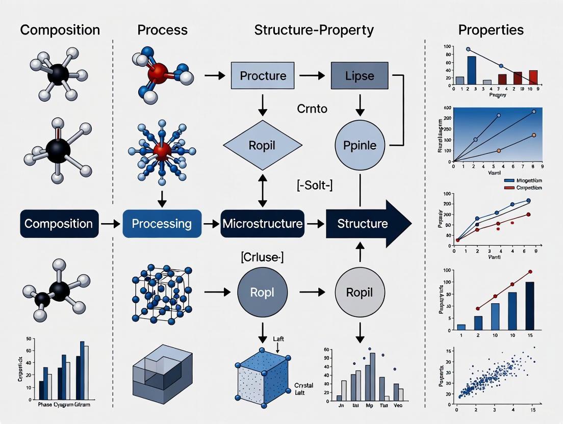
The Core Principles: Unraveling the Fundamental Links Between Composition, Processing, and Material Architecture
The Composition-Process-Structure-Property (CPSP) paradigm represents the fundamental framework of materials science and engineering, establishing the causal relationships that govern material behavior and performance. This paradigm posits that a material's ultimate properties are determined by its internal structure, which in turn is controlled by its chemical composition and processing history. Recent advances in computational modeling, machine learning, and data science have transformed this classical concept into a powerful predictive framework for inverse materials design. This technical guide examines the core principles of the CPSP paradigm, explores cutting-edge implementation methodologies across diverse material systems, and provides detailed experimental protocols for establishing robust CPSP relationships. By examining applications from dual-phase steels to high-entropy alloys and drug delivery systems, we demonstrate how the systematic decoding of CPSP linkages enables accelerated development of advanced materials with tailored properties.
The Composition-Process-Structure-Property (CPSP) paradigm serves as the central dogma of materials design, providing a systematic framework for understanding how processing conditions and chemical composition govern microstructural evolution and ultimately determine material properties and performance. This foundational principle recognizes that material behavior cannot be understood through composition alone, but rather through the intricate interrelationships between synthesis parameters, resulting microstructure, and macroscopic manifestations [1] [2].
Traditional materials development has been constrained by forward "process-structure" models that often rely on costly uncertainty quantification and trial-and-error approaches. These methods frequently falter under sparse data conditions and when confronted with complex, heterogeneous microstructures [1]. The inverse design strategy—starting from desired properties and working backward to identify optimal compositions and processing routes—represents a paradigm shift enabled by computational advances. This approach replaces traditional uncertainty quantification with direct "structure-to-process modeling," leveraging real microstructural features to map composition and processing parameters [1].
The evolution of the CPSP paradigm has been accelerated by emerging technologies in artificial intelligence, high-throughput computation, and advanced characterization. Machine learning (ML) techniques now offer powerful tools to uncover underlying patterns from experimental data and predict material properties, providing an effective approach to materials design and optimization [3] [4]. These capabilities are particularly valuable for navigating complex material systems where traditional methods face limitations due to vast compositional spaces and processing parameters [3].
Core Principles of the CPSP Framework
The Fundamental Relationships
The CPSP framework establishes hierarchical relationships between four critical elements in materials design:
- Composition: The chemical identity and proportion of constituent elements, which establishes the fundamental building blocks and potential phase equilibria.
- Processing: The synthesis and manufacturing parameters that dictate how composition transforms into structure through thermal, mechanical, or chemical pathways.
- Structure: The arrangement of material components across multiple length scales, including crystal structure, phase distribution, grain morphology, and defects.
- Properties: The resulting macroscopic behaviors and performance metrics, including mechanical, thermal, electrical, and chemical characteristics.
These relationships are not linear but form an interconnected network with feedback loops. For example, in dual-phase steels, the optimal balance between soft-phase polygonal ferrite (facilitating plastic deformation) and hard-phase martensite (imparting strength) determines mechanical properties, with processing parameters controlling this phase distribution [1]. Similarly, in high-entropy alloys (HEAs), corrosion resistance is influenced not only by chemical composition but also by microstructure and processing techniques, particularly through how crystal structure affects elemental distribution and phase stability [3].
Inverse Design Strategy
A significant advancement in CPSP implementation is the shift from forward models to inverse design strategies. Where traditional approaches follow a "process→structure→property" sequence, inverse design begins with target properties and identifies optimal structures, then determines the composition and processing routes needed to achieve them [1]. This methodology is particularly powerful for applications such as unified dual-phase (UniDP) steels, which enable tailored performance from a single composition, addressing sustainability challenges related to recyclability and weldability [1].
Table 1: Comparison of Traditional vs. Inverse Design Approaches in CPSP
| Aspect | Traditional Forward Design | Inverse CPSP Design |
|---|---|---|
| Sequence | Process → Structure → Property | Property → Structure → Process |
| Uncertainty Handling | Relies on costly uncertainty quantification | Replaces UQ with direct structure-to-process modeling |
| Computational Demand | High for complex systems | Reduced through latent space sampling |
| Data Requirements | Extensive labeled datasets | Leverages both labeled and unlabeled microstructural data |
| Primary Applications | Well-characterized material systems | Complex, multi-component systems with sparse data |
Computational Frameworks for CPSP Modeling
Machine Learning Architectures for CPSP Relationships
Modern CPSP modeling leverages sophisticated machine learning architectures to establish robust relationships across the materials design chain:
Deep Learning Integration: Advanced frameworks integrate variational autoencoders (VAE) to encode authentic microstructural features into a latent space and multilayer perceptrons (MLP) to predict composition, processing routes, and properties [1]. This architecture effectively captures the complexity of free-form microstructures and the nonlinear relationships inherent in material systems, overcoming limitations of traditional microstructural descriptors that fail to capture topological complexity and stochasticity [1].
Knowledge Graph-Driven Approaches: The Mat-NRKG model exemplifies how knowledge graphs can organize and model unstructured process-related data in flexible graph structures, capturing complex relationships among composition, processing, and structure-performance correlations [3]. This approach uses the TransE algorithm for knowledge graph completion to predict crystal structure while integrating compositional and processing information through Graph Convolutional Networks (GCN) augmented with Deep Taylor Block modules [3].
Two-Stage Prediction Frameworks: The Composition and Processing-Driven Two-Stage Corrosion Prediction Framework with Structural Prediction (CPSP Framework) hierarchically models composition–processing–structure–performance relationships [3]. This approach first predicts crystal structure from composition and processing data, then integrates this predicted structure with original inputs to forecast properties, eliminating the need for experimentally obtained structural data during inference and improving engineering applicability [3].
Framework Performance Comparison
Evaluations of different CPSP modeling approaches demonstrate distinct performance characteristics:
Table 2: Performance Comparison of CPSP Modeling Frameworks for HEA Corrosion Prediction
| Model Framework | Base Model | R² Score | MSE | MAE | Key Characteristics |
|---|---|---|---|---|---|
| CP Framework | RF | 0.641 | 0.218 | 0.381 | Composition-only baseline |
| CPP Framework | RF | 0.672 | 0.201 | 0.362 | Includes processing information |
| CPSP Framework | RF | 0.703 | 0.194 | 0.354 | Adds predicted crystal structure |
| CPSP Framework | MLP | 0.689 | 0.207 | 0.368 | Neural network implementation |
| Mat-NRKG | GCN-DTB | 0.823 | 0.146 | 0.291 | Knowledge graph integration |
| Mat-NRKGCPP | GCN-DTB | 0.672 | 0.211 | 0.349 | Ablated without structure prediction |
The CPSP Framework consistently outperforms both Composition-Only (CP) and Composition-Processing-Based (CPP) frameworks, with the knowledge graph-driven Mat-NRKG model achieving the best performance (25% improvement in MSE over the best-performing baseline) [3]. These results quantitatively demonstrate the benefit of incorporating crystal structure information into property prediction processes [3].
Experimental Protocols for CPSP Relationship Establishment
Microstructure-Driven Inverse Design Protocol
Objective: To establish inverse CPSP linkages for dual-phase steels using microstructure-centric deep learning.
Materials and Equipment:
- Dataset of microstructural images from prior studies [1]
- Data augmentation pipeline (rotation, flipping, brightness adjustment)
- Computational resources for deep learning (GPU acceleration recommended)
- Variational Autoencoder (VAE) architecture
- Multilayer Perceptron (MLP) network
- Specific latent space sampling algorithm
Procedure:
Data Preparation:
- Collect microstructural images from prior studies of dual-phase steels [1]
- Apply binarization and data augmentation to enhance quality and variability
- Curate dataset to ensure representative sampling of microstructural features
Model Architecture Implementation:
- Implement VAE to encode microstructural images into compact latent space
- Design MLP to map latent representations to composition, processing parameters, and mechanical properties
- Establish physics-informed design environment enriched by precise CPSP relationships
Training and Validation:
- Train model using combined VAE-MLP architecture
- Validate predictions against experimental results
- Apply specific latent space sampling based on principles of physical metallurgy
Inverse Design Application:
- Identify target mechanical properties for three industrial grades
- Traverse latent space to identify microstructures yielding target properties
- Determine optimal composition and processing routes to achieve identified microstructures
Experimental Validation: Synthesize designed alloys and characterize mechanical properties, comparing with predictions. Successful implementation for UniDP steels has achieved target properties across three performance tiers at lower cost than commercial alloys [1].
Knowledge Graph-Driven CPSP Protocol
Objective: To predict corrosion resistance of high-entropy alloys using the Mat-NRKG model.
Materials and Equipment:
- HEA Corrosion Resistance Dataset (HEA-CRD) with composition, processing, and corrosion current records [3]
- Knowledge graph framework
- Graph Convolutional Network (GCN) with Deep Taylor Block module
- TransE algorithm for knowledge graph completion
- PyTorch or similar deep learning environment
Procedure:
Data Curation:
- Collect corrosion resistance records from literature, encompassing composition, processing techniques, and crystal structures
- Extract and standardize processing technique descriptions
- Annotate crystal structure information
Knowledge Graph Construction:
- Organize unstructured process-related data in flexible graph structure
- Establish nodes for composition elements, processing parameters, and structural features
- Define relationships between entities based on literature evidence
Model Implementation:
- Implement TransE algorithm for knowledge graph completion to predict crystal structure
- Build GCN with DTB module to integrate compositional and processing information
- Train end-to-end model to predict corrosion current
Model Validation:
- Split data into training, validation, and test sets (4:1:1 ratio)
- Perform multiple random splits to ensure statistical significance
- Synthesize validation HEAs for experimental confirmation
Experimental Validation: The Mat-NRKG model demonstrated 25% improvement in MSE over best-performing baseline models when predicting corrosion current, with successful experimental validation on five laboratory-synthesized HEAs [3].
CPSP Visualization Frameworks
Inverse Design Workflow
CPSP Inverse Design Workflow: This diagram illustrates the inverse design approach, beginning with target properties and working backward through microstructure analysis, composition optimization, and processing parameter design, culminating in experimental validation.
Two-Stage Prediction Framework
Two-Stage CPSP Prediction: This visualization represents the two-stage prediction framework that first predicts crystal structure from composition and processing parameters, then integrates this information for final property prediction.
Research Reagent Solutions for CPSP Studies
Table 3: Essential Research Reagents and Materials for CPSP Investigations
| Reagent/Material | Function in CPSP Research | Example Applications |
|---|---|---|
| Dual-Phase Steel Systems | Model material for establishing microstructure-property relationships | Unified dual-phase (UniDP) steel development [1] |
| High-Entropy Alloys (Al-Co-Cr-Fe-Cu-Ni-Mn) | Complex composition systems for corrosion resistance studies | CPSP framework validation for corrosion prediction [3] |
| Poly(Lactide-co-Glycolide) (PLGA) | Biopolymer for drug delivery system studies | Long-acting injectables development [4] |
| Variational Autoencoder (VAE) | Microstructural feature encoding into latent space | Inverse design of dual-phase steels [1] |
| Graph Convolutional Network (GCN) | Knowledge graph processing for materials data | Mat-NRKG model for HEA corrosion prediction [3] |
| TransE Algorithm | Knowledge graph completion for structure prediction | Crystal structure prediction from composition/processing [3] |
The CPSP paradigm represents the foundational framework for modern materials design, enabling accelerated development of advanced materials through systematic decoding of composition-process-structure-property relationships. The integration of machine learning, knowledge graphs, and inverse design strategies has transformed this classical materials science concept into a powerful predictive framework capable of navigating complex, multi-dimensional design spaces. The experimental protocols and computational frameworks presented herein provide researchers with robust methodologies for implementing CPSP-driven materials design across diverse material systems, from structural metals to functional polymers. As computational power advances and datasets expand, the CPSP paradigm will continue to evolve, offering increasingly sophisticated approaches for inverse materials design and accelerating the development of next-generation materials with tailored properties and enhanced performance.
Within the framework of composition-process-structure-property (CPSP) relationships research, the elemental composition of a material is a primary determinant of its final characteristics. It directly dictates the stable crystal phases that form during processing and governs the intrinsic properties—mechanical, magnetic, functional—that the material will exhibit. This foundational principle is critical for the goal-oriented design of advanced materials, from high-performance alloys to functional compounds. Moving beyond traditional trial-and-error methods, modern research leverages combinatorial experiments and data-driven modeling to unravel these complex relationships, enabling the precise inverse design of materials tailored for specific applications [5] [6] [1].
Core Principles: Composition and Phase Stability
The elemental composition of a material system establishes its fundamental thermodynamic landscape, which in turn dictates phase formation. A key manifestation of this principle is observed in High Entropy Alloys (HEAs), multi-principal element systems where the concentration of each element can be strategically varied to tailor structure and properties [5].
The Al Composition Dictates Crystal Structure
Research on the FeMnCoCrAl system demonstrates that varying the concentration of a single element, such as aluminum, can trigger complete phase transitions. The equiatomic FeMnCoCr base alloy (0 at.% Al) crystallizes in the complex α-Mn structure. However, introducing Al additions causes a shift to a more stable Body-Centered Cubic (BCC) random solid solution [5].
Table 1: Effect of Al Composition on Phase Formation in FeMnCoCrAl Thin Films [5]
| Aluminum Content (at.%) | Crystal Structure Evolution | Key Observations |
|---|---|---|
| 0 | α-Mn | Base alloy structure. |
| 4 | α-Mn + BCC | BCC phase begins to form. |
| 6 | BCC (dominant) | BCC phase becomes predominant. |
| 8 | Single BCC | Single-phase random solid solution; lattice parameter = 2.88 Å. |
| 20 - 38 | BCC | Lattice parameter increases with Al content (up to 1.04%). |
| 40 | BCC + B2 | Appearance of an ordered B2 (superlattice) phase. |
| >50 | Low Crystallinity | Broad, low-intensity XRD peaks; suggests amorphization. |
This structural evolution is consistent with density functional theory (DFT) predictions, which indicate that Al additions increase the stability of the BCC phase over the Face-Centered Cubic (FCC) phase, a phenomenon rationalized by the formation of a pseudogap at the Fermi level [5].
Impact of Composition on Intrinsic Properties
Elemental composition directly controls intrinsic properties by altering the electronic structure and atomic-level interactions within a material. A prime example is the manipulation of magnetic properties through compositional changes.
Magnetic Properties
In the paramagnetic FeMnCoCr base alloy, the addition of Al induces ferromagnetism. The saturation magnetization (Ms) does not increase monotonically; it reaches a maximum at a specific critical composition of 8 at.% Al and then decreases as the concentration of non-ferromagnetic Al is increased further. This trend is consistent with ab initio predictions of the Al concentration-induced changes in the magnetic moment [5].
Table 2: Al Composition and Resulting Magnetic Properties in FeMnCoCrAl [5]
| Aluminum Content (at.%) | Magnetic Behavior | Saturation Magnetization (Ms) |
|---|---|---|
| 0 | Paramagnetic | - |
| 8 | Ferromagnetic | Maximum |
| > 8 | Ferromagnetic | Concomitant decrease |
| > 40 | Not Reported | Not Reported |
The initial increase in Ms is attributed to the Al-driven phase transition to the BCC structure, which favors ferromagnetic ordering. The subsequent decrease beyond 8 at.% Al is due to a reduction in the number density of ferromagnetic species (Fe and Co) as they are progressively replaced by non-ferromagnetic Al [5].
Experimental and Computational Methodologies
Establishing robust CPSP links requires sophisticated experimental and computational protocols.
Combinatorial Thin-Film Synthesis & High-Throughput Characterization
This efficient methodology involves depositing compositionally graded thin-film libraries to explore a wide composition space in a single experiment [5].
- Experimental Protocol (FeMnCoCrAl Study) [5]:
- Deposition: Five separate FeMnCoCrAl thin-film spreads are deposited with Al concentration gradients ranging from 3.5 to 54.0 at.%.
- Composition Verification: The chemical composition across the library is characterized using Energy Dispersive X-ray (EDX) analysis.
- Phase Identification: X-ray diffraction (XRD) is used to map the phase formation and lattice parameter evolution as a function of Al content.
- Microstructural Analysis: Atom probe tomography (APT) is employed to probe the local chemical composition and distribution of elements at the atomic scale, confirming the formation of a random solid solution without segregation.
Data-Driven and Inverse Design Modeling
To overcome the limitations of costly experiments and high-fidelity simulations, machine learning models are increasingly used to decode PSP relationships [6]. A leading-edge approach is microstructure-centric inverse design, which inverts the traditional "process-structure" paradigm [1].
- Computational Protocol (Unified Dual-Phase Steel Design) [1]:
- Data Curation: A dataset of microstructural images is collected and pre-processed through binarization and data augmentation.
- Feature Encoding: A variational autoencoder (VAE) is used to encode the high-dimensional microstructural images into a compact, low-dimensional latent space representation.
- Property & Process Mapping: A multilayer perceptron (MLP) maps the latent microstructural representation to the corresponding composition, processing parameters, and mechanical properties, establishing a direct "structure-to-process" link.
- Inverse Design: By sampling the trained latent space, new microstructures that yield target properties can be generated, and the inverse model directly recommends the composition and processing needed to achieve them.
Visualizing Composition-Structure-Property Relationships
The complex relationships between composition, structure, and properties can be visualized as an interconnected workflow, encompassing both experimental and computational pathways.
Diagram 1: The CPSP relationships workflow, showing both forward (experimental) and inverse (data-driven) design pathways.
The Scientist's Toolkit: Essential Research Reagents and Materials
Table 3: Key Reagents and Materials for Composition-Property Research
| Item / Technique | Function in Research |
|---|---|
| Combinatorial Thin-Film Library | A high-throughput platform for synthesizing a continuous gradient of compositions on a single substrate, enabling rapid screening of phase formation and properties [5]. |
| Energy Dispersive X-ray (EDX) Analysis | Used for precise quantitative analysis of the local chemical composition across the material library [5]. |
| X-ray Diffraction (XRD) | A fundamental technique for identifying crystal structures, phases, lattice parameters, and detecting ordering or amorphization [5]. |
| Atom Probe Tomography (APT) | Provides three-dimensional, atomic-scale resolution mapping of the distribution of all elements within a material, confirming solid solution formation or revealing segregation [5]. |
| Vibrating Sample Magnetometer (VSM) / SQUID | Instruments used to measure the magnetic properties of a material, such as saturation magnetization and coercivity [5]. |
| Variational Autoencoder (VAE) | A type of generative machine learning model that encodes complex microstructural images into a lower-dimensional latent space for analysis and inverse design [1]. |
| Multilayer Perceptron (MLP) | A foundational neural network architecture used to establish predictive relationships between encoded microstructures, processing parameters, and final properties [1]. |
Within additive manufacturing (AM) and advanced materials processing, the established composition-process-structure-property (CPSP) relationship is paramount. This technical review posits that thermal cycles, energy input, and fabrication routes act as fundamental architectural elements that directly govern microstructural evolution. Through layer-by-layer fabrication, materials undergo complex thermal histories that trigger solid-state phase transformations, segregation phenomena, and grain restructuring, ultimately dictating the mechanical properties of the final component. This paper synthesizes recent research to provide an in-depth analysis of these relationships, offering a structured guide to the experimental methodologies and data-driven models that are shaping the future of microstructural design.
In traditional manufacturing, process parameters are typically designed to achieve a single set of microstructural characteristics. In contrast, additive manufacturing and similar advanced processes introduce a dynamic thermal landscape where the fabrication route itself becomes an active design variable. The concept of "Processing as the Architect" emerges from the ability to precisely control these thermal cycles to elicit specific microstructural responses from a single material composition.
The sequential nature of these processes means that previously deposited material is subjected to repeated heating and cooling cycles as new layers are added. This intrinsic heat treatment (IHT) leads to a non-equilibrium microstructure that cannot be replicated through conventional means. The following sections deconstruct the core mechanisms of this architectural control, providing quantitative data, experimental protocols, and visualizations of the underlying relationships.
Core Architectural Elements
Thermal Cycles as Microstructural Modulators
Thermal cycles during layered fabrication act as an in-situ heat treatment, profoundly altering microstructure. In laser-directed energy deposition (LDED) of GA151K Mg alloy, thermal cycles cause two significant solid-phase transformations: the intergranular phase changes from Mg3Gd to Mg5Gd, and fine β'-Mg7Gd precipitates form within the α-Mg matrix from a supersaturated solid solution [7]. These transformations are directly linked to changes in mechanical properties, with microhardness increasing by 6.9 ± 5.0 HV0.2 in areas experiencing more thermal cycles [7].
Similarly, in wire-based electron beam directed energy deposition (EB-DED) of nickel-based superalloys, thermal cycling creates an altered morphology along the build height and promotes the formation of Nb-rich interdendritic zones [8]. The thermal history determines the precipitation behavior of strengthening phases (γ" and δ), with longer deposition times favoring fine γ" precipitation throughout the build height [8].
Table 1: Microstructural Transformations Induced by Thermal Cycles in Different Alloy Systems
| Alloy System | AM Process | Phase Transformations | Microstructural Effects | Property Changes |
|---|---|---|---|---|
| GA151K (Mg-Gd) [7] | Laser-DED | Mg3Gd → Mg5Gd; Precipitation of β'-Mg7Gd | Reduced fraction of island-like intergranular phase (↓9.3±2.1%) | Microhardness increased by 6.9±5.0 HV0.2 |
| Nickel-based Superalloy [8] | Wire-based EB-DED | Precipitation of γ" and δ phases | Heterogeneous γ" distribution along build height; Nb segregation in interdendritic zones | Graded mechanical properties along build direction |
| X70 Pipeline Steel [9] | Laser-DED | Precipitation of Fe3C; Dislocation density reduction | Grain coarsening from bottom to top; Increased polygonal ferrite | Decreasing microhardness along building direction |
Energy Input as a Governing Parameter
Energy input, quantified as Energy Area Density (EAD) or Energy Volume Density (EVD), directly controls thermal profiles and resulting microstructure. In selective laser melting (SLM) of low-alloy steel, increasing EAD from 47 to 142 J/mm² transforms the microstructure from a mixture of lower bainite and martensite-austenite to granular bainite, while remarkably reducing grain size from 6.31 μm to 1.56 μm [10].
For L-DED repaired X70 steel, the energy input calculation follows:
EVD = P / (v * d * h)
where P is laser power (W), v is scanning speed (mm/min), d is laser spot diameter (mm), and h is layer height (mm). With an EVD of 50 J/mm³, this process produces microstructural inhomogeneity along the building direction, with grains gradually coarsening and polygonal ferrite proportion increasing from bottom to top [9].
Table 2: Energy Input Parameters and Their Microstructural Effects in Metal AM
| Material | AM Process | Energy Parameter | Value Range | Microstructural Effects | Grain Size (μm) |
|---|---|---|---|---|---|
| Low-alloy Steel [10] | Selective Laser Melting | Energy Area Density (EAD) | 47-142 J/mm² | Mixed lower bainite/martensite → Granular bainite; Bainite ferrite: lath → multilateral | 6.31 @ 47 J/mm²; 1.56 @ 142 J/mm² |
| X70 Steel [9] | Laser-DED | Energy Volume Density (EVD) | 50 J/mm³ | Grain coarsening bottom to top; Increased polygonal ferrite; Fe3C precipitation | Inhomogeneous along build direction |
| GA151K Mg Alloy [7] | Laser-DED | Not specified | Not specified | Intergranular phase transformation; β' precipitation within α-Mg matrix | Fine α-Mg grains (size not specified) |
Fabrication Routes and Thermal Management Strategies
The specific fabrication route and thermal management strategy employed during manufacturing significantly influence the resulting thermal history and microstructure. Research on nickel-based superalloys demonstrates that a discontinuous interpass cooling strategy (ICS) produces homogeneous mechanical properties throughout the build, while a continuous deposition strategy (CDS) results in graded mechanical properties and decreasing strength along the build height due to heterogeneous γ" distribution [8].
The scanning strategy also plays a crucial role. A zigzag scanning pattern with 45% overlap between adjacent tracks was utilized in SLM of low-alloy steel to ensure proper fusion while controlling thermal accumulation [10]. Similarly, L-DED of X70 steel employed a "layered reciprocating scanning strategy" to build 40×40×4.5 mm samples [9].
Experimental Protocols for Microstructural Analysis
Sample Preparation and Metallography
Standard metallographic procedures are essential for accurate microstructural characterization. For LDED GA151K Mg alloy, samples were prepared through mechanical grinding and polishing, with final etching using a solution of 5 mL HNO3 + 95 mL C2H5OH for approximately 10 seconds [10]. For EBSD analysis, electropolishing with 8 mL HClO4 + 92 mL C2H5OH at -15°C for 15 seconds was employed [10].
Microstructural characterization typically utilizes multiple complementary techniques:
- Optical Microscopy (OM) and Scanning Electron Microscopy (SEM) for general microstructural observation [10] [9]
- Electron Backscatter Diffraction (EBSD) for grain morphology and size analysis [10]
- Transmission Electron Microscopy (TEM) for substructure and fine precipitate characterization [10]
Thermal Cycle Monitoring and Analysis
Understanding thermal history is crucial for correlating process parameters with microstructure. Finite element method (FEM) simulations can model the evolution of the temperature field during manufacturing [10]. For accurate simulations, thermal physical properties must be experimentally measured below certain temperatures (e.g., 900°C) and calculated using specialized software like JMATPRO for higher temperatures [10].
Phase transformation temperatures can be experimentally determined using a thermal expansion tester with specific heating and cooling rates (e.g., 10°C/s heating and 5°C/s cooling) [10].
Mechanical Property Evaluation
Standard mechanical tests correlate microstructural features with performance:
- Microhardness testing (e.g., HV0.2) across different regions reveals property variations [7] [9]
- Tensile testing at room temperature (e.g., 0.6 mm/min) evaluates yield strength, ultimate tensile strength, and elongation [10] [9]
- Fracture surface analysis via SEM identifies fracture mechanisms (ductile vs. brittle) [10]
Data-Driven Modeling of Process-Structure-Property Relationships
Traditional physics-based modeling of PSP relationships faces challenges due to computational costs and complex multi-physics phenomena [6]. Data-driven approaches have emerged as powerful alternatives:
Machine Learning Frameworks
Gaussian process regression effectively models nonlinear relationships between process parameters and resulting features like molten pool geometry, requiring relatively small datasets [6]. This approach has successfully predicted molten pool depth in LPBF and identified parameter combinations for desirable conduction mode melting versus keyhole mode [6].
Variational autoencoders (VAE) can encode microstructural images into a latent space representation, while multilayer perceptrons (MLP) map this representation to composition, processing parameters, and mechanical properties [1]. This microstructure-centric inverse design strategy has successfully developed unified dual-phase (UniDP) steels that achieve target properties across multiple performance tiers from a single composition [1].
Microstructural Quantification Methods
Data-driven modeling relies on quantitative microstructural descriptors:
- Simplified descriptors: Phase fractions, grain size, morphological parameters [1]
- Complex descriptors: 2-point statistics, N-point statistics, and machine learning-derived features [1]
Generative models like VAEs and generative adversarial networks (GANs) effectively capture free-form microstructural complexity and nonlinear relationships in material systems [1].
The Scientist's Toolkit: Essential Research Reagents and Materials
Table 3: Key Research Materials and Equipment for Thermal Cycle-Microstructure Studies
| Item Category | Specific Examples | Function/Application | Research Context |
|---|---|---|---|
| Base Materials | GA151K Mg alloy powder (Mg-15Gd-1Al-0.4Zr) [7] | LDED feedstock for studying phase transformations | Mg-RE alloy microstructural evolution under thermal cycles |
| Low-alloy steel powder (C: 0.15-0.25%, Mn: 0.6%, Ni: 1.0%, Mo: 0.5%) [10] | SLM feedstock for bainitic/martensitic transformation studies | Effect of EAD on microstructure in ferrous alloys | |
| X70 pipeline steel powder [9] | L-DED repair feedstock | Repair processes and microstructural inhomogeneity | |
| Characterization Equipment | Field Emission SEM (e.g., Nova NanoSEM50) [10] | High-resolution microstructural imaging | General microstructural characterization |
| EBSD System [10] | Grain morphology and orientation analysis | Crystallographic texture and grain size measurement | |
| Transmission Electron Microscope [10] | Fine precipitate and substructure analysis | Nanoscale precipitation characterization | |
| Process Monitoring | Thermal Expansion Tester [10] | Phase transformation temperature measurement | Determination of critical transformation temperatures |
| Finite Element Modeling Software | Temperature field simulation | Thermal history prediction | |
| Chemical Reagents | Nitric Acid Alcohol Etchant (4% HNO3 in C2H5OH) [9] | Microstructural etching for ferrous alloys | Revealing grain boundaries and phases |
| Electrolyte for Electropolishing (8% HClO4 in C2H5OH) [10] | Sample preparation for EBSD | Creating deformation-free surfaces for diffraction |
Visualization of Process-Microstructure Relationships
Microstructural Architecture Pathway: This diagram illustrates how process parameters govern thermal history, which in turn dictates microstructural evolution and final mechanical properties.
Experimental Workflow: This diagram outlines the comprehensive methodology for investigating thermal cycle effects on microstructure, from sample fabrication through characterization to final data analysis.
The architectural role of processing parameters—specifically thermal cycles, energy input, and fabrication routes—in defining microstructure is now firmly established within materials science research. The evidence demonstrates that these factors directly control phase transformations, precipitation behavior, grain evolution, and elemental segregation across diverse alloy systems.
Future research directions will likely focus on several key areas:
- Advanced thermal management strategies that provide finer control over thermal histories during fabrication
- Integrated computational materials engineering (ICME) approaches that combine multi-scale modeling with experimental validation
- Machine learning-enhanced inverse design methodologies that accelerate the development of materials with tailored properties [1] [6]
The understanding that "processing architects microstructure" provides a powerful framework for designing next-generation materials with spatially graded properties optimized for specific application requirements. This paradigm shift from passive processing to active microstructural design promises to revolutionize materials development across aerospace, automotive, energy, and biomedical sectors.
In the foundational paradigm of composition-process-structure-property relationships, microstructure serves as the pivotal, though often complex, link between how a material is made and how it performs. Microstructure refers to the spatial arrangement and connectivity of internal constituents—such as grains, pores, and phases—at length scales ranging from nanometers to micrometers [11]. Unlike inherent molecular structures, microstructures are emergent properties formed during manufacturing and processing, making their quantification essential for predicting and controlling final product attributes [11]. In pharmaceuticals, microstructure determines Critical Quality Attributes (CQAs) like drug release, stability, and content uniformity [12] [13]. In metallurgy, it governs mechanical properties such as hardness and strength [14] [6]. This technical guide details the evolution of microstructure quantification from simple, low-order descriptors to sophisticated spatial statistics and AI-driven characterization, providing researchers with methodologies to elucidate these critical process-structure-property relationships.
Foundational Microstructural Descriptors
Initial microstructure characterization relies on low-order metrics that provide global averages but lack detailed spatial information.
Table 1: Foundational Microstructural Descriptors and Their Limitations
| Descriptor Category | Specific Metrics | Applications | Key Limitations |
|---|---|---|---|
| Global Composition | Volume fraction, phase fraction | Ti6Al4V analysis [15], PLGA microspheres [12] | Does not capture spatial distribution |
| Basic Morphology | Grain size, particle size, alpha colony size [15], porosity, surface area [13] | Quality control, initial screening | Lacks information on spatial clustering or connectivity |
| Dispersion Form | Crystalline vs. amorphous state, domain size [12] | Predicting drug release kinetics [12] | Does not describe location within the matrix |
While these descriptors are invaluable for quality control and establishing baseline comparisons (e.g., Q1/Q2 similarity in generics [12]), they are insufficient for predicting complex properties like fracture toughness or controlled drug release, which are highly dependent on the spatial arrangement of microstructural features.
Statistical Microstructural Descriptors (SMDs) for Spatial Quantification
To move beyond averages, the field employs Statistical Microstructural Descriptors (SMDs)—mathematical functions that quantify the spatial arrangement and correlation of features.
Two-Point Correlation Functions
The two-point correlation function, ( P_{11}(r) ), is a fundamental SMD defined as the probability that two points separated by a vector ( r ) lie in the same phase of interest (e.g., a particle or pore) [16]. Its orientation-averaged version, estimated from metallographic sections, reveals the degree of spatial clustering [16]. Applications include quantifying clustering in SiC-reinforced aluminum composites, where extracted length scales from the correlation function directly correlate with processing parameters like particle size ratio and extrusion ratio [16].
Higher-Order Spatial Correlations
Two-point statistics have limitations, as different microstructures can share the same two-point correlation [17]. Higher-order descriptors are needed to uniquely characterize complex systems.
- n-Point Statistics and Polytope Functions: These capture complex morphological information, such as the probability of finding n vertices of a specific polytope (e.g., a triangle or square) within a given phase [17]. They are more powerful for reconstructing and distinguishing complex, multi-scale microstructures.
- Ripley's K and L Functions: Derived from spatial statistics, these functions assess if features exhibit a random, dispersed, or clustered distribution at a specific spatial scale [18]. The L function, ( \hat{L}(t) ), is a variance-stabilized version of the K function. For homogeneous data, ( \hat{L}(t) ) has an expected value of ( t ), and a plot of ( t - \hat{L}(t) ) against ( t ) helps identify deviations from spatial randomness [18].
Fractal Descriptions for Multi-Scale Heterogeneity
Fractal analysis describes how observed variance or heterogeneity changes with the scale of measurement. It is particularly useful for systems exhibiting self-similarity over a range of length scales. The core relationship is a power law:
[ RD(m) = RD(m0) \left( \frac{m}{m0} \right)^{1-D} ]
where ( RD(m) ) is the relative dispersion (coefficient of variation) at a measurement scale of mass ( m ), ( m_0 ) is a reference mass, and ( D ) is the fractal dimension [19]. This dimension provides a measure of spatial correlation, with specific bounds indicating randomness (( D = 1.5 )) or perfect uniformity (( D = 1.0 )) [19].
The following diagram illustrates the workflow for applying these spatial statistics to quantify a microstructure, from image acquisition to interpretation.
Figure 1: Workflow for Spatial Statistical Analysis of Microstructure
Experimental Protocols for Microstructure Quantification
Automated 2D Microstructural Analysis Protocol
This protocol, validated on Ti6Al4V, enables high-throughput, repeatable quantification of features like grain size and volume fraction of globular alpha grains [15].
- Image Acquisition: Obtain high-resolution 2D images via Scanning Electron Microscopy (SEM) or Optical Microscopy.
- Digital Image Processing: Apply algorithms to isolate individual microstructural features (e.g., grains, colonies).
- Image Segmentation: Use techniques like the watershed algorithm to partition the image into regions representing distinct microstructural entities.
- Morphological Measurement: Extract quantitative data (size, shape, volume fraction) from the segmented regions.
- Validation: Compare results with manual measurements to ensure consistency while achieving drastically improved speed and repeatability [15].
Protocol for 3D Two-Point Correlation Function Estimation
This stereological method allows for unbiased estimation of 3D spatial correlations from 2D vertical sections, crucial for understanding anisotropic microstructures [16].
- Vertical Section Sampling: Identify a symmetry axis (e.g., from an extrusion process). Section the sample along a plane containing this axis.
- Digital Image Montage: Capture a large, high-resolution montage of micrographs from the vertical section to ensure a representative field of view and minimize edge effects.
- Unbiased Lineal Measurement: Using digital image analysis, place test lines of varying length and orientation across the montage. For each line length ( r ), count the fraction where both endpoints lie in the phase of interest.
- Orientation Averaging: Compute the orientation-averaged mean two-point correlation function, ( \langle P_{ij}(r) \rangle ), by integrating measurements over all spatial directions, weighted by ( \sin \theta ) [16].
- Length Scale Extraction: Analyze the resulting correlation function to identify characteristic length scales of clustering, such as the distance at which the function plateaus to its long-range value.
The Scientist's Toolkit: Essential Reagents and Materials
Successful microstructural quantification relies on a suite of advanced analytical techniques and computational tools.
Table 2: Key Research Reagent Solutions for Microstructure Characterization
| Tool Category | Specific Technology | Primary Function in Microstructure Analysis |
|---|---|---|
| Advanced Microscopy | Scanning Electron Microscopy (SEM) [15] [11], Focused Ion Beam-SEM (FIB-SEM) [12], Confocal Laser Scanning Microscopy (CLSM) [12] | High-resolution 2D and 3D imaging of surface and sub-surface features. |
| 3D & Chemical Imaging | X-ray Microscopy (XRM) [12], Synchrotron Radiation X-ray μCT (SR-μCT) [12] [17], Confocal Raman Microscopy (CRM) [12] [11] | Non-destructive 3D volumetric imaging; mapping of chemical composition and component distribution. |
| Surface & Spectral Analysis | Time-of-Flight Secondary Ion Mass Spectrometry (ToF-SIMS) [12], Atomic Force Microscopy (AFM) [11], Energy Dispersive Spectroscopy (EDS) [12] | Elemental and isotopic surface mapping; nanoscale topographic imaging. |
| AI & Image Analytics | Generative Adversarial Networks (GANs) [17], Deep Convolutional Neural Networks [17] [6], Digital Image Processing Algorithms [15] [13] | Automated segmentation, feature measurement, and synthetic microstructure reconstruction. |
Advanced & Emerging Methodologies: AI and Multi-Scale Reconstruction
The frontier of microstructure quantification lies in integrating AI and higher-order statistics to overcome imaging limitations and discover new PSP relationships.
Deep Generative Models for Microstructure Reconstruction
Generative Adversarial Networks (GANs), such as Deep Convolutional GAN (DCGAN) and StyleGAN2, are used to synthetically generate statistically equivalent, high-resolution, and potentially 3D microstructures from limited 2D image data [17]. This addresses the critical trade-off between resolution and field of view in imaging technologies. The performance of these models is evaluated by comparing higher-order SMDs (e.g., n-point polytope functions) of the original and synthetic images, ensuring morphological equivalence beyond what two-point correlations can achieve [17].
Data-Driven Modeling of Process-Structure-Property Relationships
Machine learning (ML) is revolutionizing the establishment of high-dimensional PSP linkages. For instance, neural networks have been applied to map process parameters (e.g., laser power, scan speed) to structural indicators (e.g., grain size, porosity) and finally to properties (e.g., hardness, electrical resistivity) in Pt-Au nanocrystalline alloys [14] and metal additive manufacturing [6]. These models can rapidly identify optimal process windows to maximize material performance, a task that is prohibitively time-consuming using purely experimental or physics-based simulation approaches.
The following diagram summarizes this advanced, closed-loop framework for materials development, which integrates characterization, data science, and modeling.
Figure 2: AI-Enhanced Process-Structure-Property Framework
The journey from simplified descriptors to complex spatial statistics represents a paradigm shift in our ability to quantify microstructure. This evolution, powered by advancements in spatial statistics like two-point and n-point correlation functions and accelerated by AI and machine learning, is transforming microstructure from a qualitative micrograph into a rich, quantitative dataset. This quantitative description is the indispensable key to unlocking a fundamental, predictive understanding of composition-process-structure-property relationships. As these techniques continue to mature, they pave the way for the inverse design of materials and pharmaceutical products, enabling researchers to specify a target property and computationally design the optimal microstructure and manufacturing process to achieve it.
Dual-Phase (DP) steels, classified as first-generation Advanced High-Strength Steels (AHSS), have become indispensable materials in modern automotive engineering due to their exceptional combination of high strength and good ductility [20]. These properties are crucial for manufacturing vehicle components that enhance fuel efficiency through lightweighting while maintaining passenger safety [20]. The fundamental characteristic of DP steels is their composite-like microstructure consisting of a soft ferrite matrix with dispersed hard martensite islands, typically comprising 10-40 vol.% martensite [21]. This unique microstructure results in continuous yielding, high initial work hardening rates, and excellent energy absorption properties [21] [22].
This case study explores the intricate composition-process-structure-property relationships in DP steels, focusing specifically on how precise microstructural control enables tailoring of mechanical performance for specific applications. Understanding these relationships is paramount for researchers and engineers seeking to develop next-generation materials that meet increasingly stringent automotive requirements, particularly with the transition toward electric vehicles that demand optimized weight-to-strength ratios for extended battery range [23].
Microstructural Fundamentals of Dual-Phase Steels
Phase Characteristics and Their Roles
The mechanical behavior of DP steels derives from the synergistic interaction between its two constituent phases:
Ferrite Matrix: This body-centered cubic (BCC) iron phase is soft and ductile, contributing primarily to the material's formability and toughness. The ferrite phase typically contains a high density of mobile dislocations, particularly near phase boundaries, which facilitates continuous yielding without a pronounced yield point elongation [20] [21].
Martensite Islands: This hard, body-centered tetragonal (BCT) phase forms via diffusionless transformation from austenite during rapid cooling. The martensite islands act as strengthening components, enhancing strength and resistance to deformation. The carbon content in martensite significantly influences its hardness and the overall strength of the DP steel [20].
A critical microstructural feature is the ferrite-martensite interface, where a high density of geometrically necessary dislocations (GNDs) accumulates due to volume expansion (2-4%) during the austenite-to-martensite transformation [20] [21]. These GNDs are mobile and contribute significantly to the initial strain hardening behavior and continuous yielding phenomenon characteristic of DP steels [20].
Key Microstructural Parameters
Three primary microstructural characteristics govern the mechanical properties of DP steels:
- Ferrite Grain Size (FGS): The size of the ferrite grains in the matrix, which follows the Hall-Petch relationship for strengthening [21].
- Martensite Volume Fraction (MVF): The proportion of martensite in the microstructure, typically ranging from 10% to 40% [21].
- Martensite Morphology (MM): The spatial distribution, size, shape, and connectivity of martensite islands [20].
Advanced characterization techniques, particularly three-dimensional EBSD (3D EBSD) conducted via tomographic serial sectioning, have revealed the complex three-dimensional distribution of these phases, providing crucial insights for microstructure-property modeling [21].
Alloying Design and Compositional Control
The chemical composition of DP steels is carefully designed to achieve the desired microstructure after specific thermal processing. Each alloying element plays a distinct role in phase transformation kinetics and final properties [21].
Table 1: Key Alloying Elements in Dual-Phase Steels and Their Functions
| Element | Typical Content (wt.%) | Primary Function | Secondary Effects |
|---|---|---|---|
| Carbon | 0.06-0.15% [21] | Austenite stabilizer; determines martensite hardness | Strengthens martensite; controls phase distribution |
| Manganese | 1.5-3.0% [21] | Austenite stabilizer; retards ferrite formation | Solid solution strengthener in ferrite |
| Silicon | ~0.5-1.0% (inferred) | Promotes ferritic transformation | Enhances carbon enrichment of austenite |
| Chromium/Molybdenum | Up to 0.4% [21] | Retards pearlite and bainite formation | Increases hardenability |
| Microalloying (V, Nb) | Trace amounts [21] | Precipitation strengthening; grain refinement | Inhibits recrystallization; improves toughness |
Carbon content is particularly critical as it directly influences the martensite volume fraction and hardness. Manganese, silicon, chromium, and molybdenum collectively control the transformation kinetics during cooling, enabling the formation of the desired ferrite-martensite microstructure without unwanted phases like pearlite or bainite [21]. Microalloying with vanadium or niobium enables precipitation strengthening and grain refinement through the formation of carbonitrides that pin grain boundaries during processing [21].
Processing Routes for Microstructural Control
The microstructure of DP steels is primarily achieved through carefully designed thermal and thermomechanical processing routes. The fundamental principle involves intercritical annealing in the (α + γ) two-phase region followed by controlled cooling to transform the austenite to martensite.
Fundamental Processing Routes
Two primary processing methods are employed industrially:
Hot-Rolled DP Steels: Produced by controlled cooling from the austenite phase after hot rolling. The process involves cooling to the intercritical region to form ferrite before rapid quenching transforms remaining austenite to martensite [21].
Cold-Rolled and Annealed DP Steels: Produced by intercritical annealing of cold-rolled sheet in the two-phase ferrite plus austenite region, followed by rapid cooling to transform austenite to martensite [21]. This route typically provides better surface quality and dimensional control.
Advanced Thermomechanical Processing
Researchers have developed advanced processing techniques to achieve ultrafine-grained (UFG) DP steels with enhanced strength-ductility combinations:
Advanced Thermomechanical Processing (ATMP): Includes methods like deformation-induced ferrite transformation (DIFT), large strain warm deformation (LSWD), intercritical hot rolling, and multi-directional rolling [21]. These techniques are suitable for commercial-scale production.
Severe Plastic Deformation (SPD): Comprises methods such as equal-channel angular pressing (ECAP), accumulative roll bonding (ARB), and high-pressure torsion [21]. These techniques can produce ferrite grain sizes of approximately 1 μm but are generally confined to laboratory-scale samples.
A typical two-step processing route for UFG DP steels involves: (1) a deformation treatment to produce UFG ferrite with finely dispersed cementite or pearlite, followed by (2) short intercritical annealing in the ferrite/austenite two-phase field and quenching to transform austenite to martensite [21].
Quantitative Property-Structure Relationships
The mechanical properties of DP steels can be quantitatively correlated with the key microstructural parameters through established relationships.
Table 2: Effect of Microstructural Parameters on Mechanical Properties of DP Steels
| Microstructural Parameter | Effect on Strength | Effect on Ductility | Effect on Strain Hardening | Typical Property Range |
|---|---|---|---|---|
| Martensite Volume Fraction (Increase from 10% to 40%) | Significant increase [21] | Moderate decrease [21] | Increase at low strains [20] | UTS: 400-1200 MPa [21] |
| Ferrite Grain Size (Refinement from 12μm to 1μm) | Increase (Hall-Petch) [21] | Slight decrease or maintained [21] | Significant increase [21] | YS: 300-1000 MPa [20] |
| Martensite Carbon Content (Increase) | Increase (martensite strength) [24] | Variable | Moderate effect | Dictates martensite hardness [24] |
| Martensite Morphology (Banded to Dispersed) | Minor effect | Significant improvement [20] | More uniform deformation | Improved hole expansion capacity [21] |
These relationships enable materials engineers to tailor the mechanical performance of DP steels for specific applications. For instance, automotive components requiring high crash resistance benefit from higher martensite volume fractions and refined ferrite grain sizes, which simultaneously increase strength and strain hardening capacity [20].
Experimental Tempering Study
Tempering of DP steels represents an important secondary processing step that modifies the as-quenched microstructure. Recent research has systematically modeled the microstructural evolutions and mechanical properties during tempering of DP steels between 100°C and 550°C [24]. The study identified:
- Two distinct tempering stages: The first stage involves cementite precipitation, while the second stage includes cementite spheroidization and recovery phenomena [24].
- Manganese content effect: Increasing manganese content retards the second tempering stage but does not significantly affect the first stage [24].
- Modeling approach: A JMAK (Johnson-Mehl-Avrami-Kolmogorov) model was developed to predict microstructural evolution during tempering, combined with a Hybrid-mean Field Composite model to predict tensile curves [24].
This modeling approach successfully reproduced the effects of tempering parameters across a wide range of microstructural conditions, providing valuable tools for industrial heat treatment design [24].
Experimental Protocols for Microstructural Control
Protocol: Intercritical Annealing for DP Microstructure Generation
Objective: To produce a dual-phase microstructure with controlled martensite volume fraction and ferrite grain size.
Materials and Equipment:
- Cold-rolled low-carbon steel sheet (C: 0.1 wt%, Mn: 1.8 wt%, Si: 0.4 wt%)
- Salt bath or tube furnace with protective atmosphere (e.g., nitrogen or argon)
- Quenching system (water or oil quench)
- Metallographic preparation equipment
- Hardness tester and tensile testing machine
Procedure:
- Cut specimens to appropriate dimensions (e.g., 150 × 30 × 1.5 mm)
- Heat treatment in single-phase austenite region at 900°C for 5 minutes for complete austenitization
- Cool to intercritical annealing temperature (e.g., 740-800°C) at a controlled rate of 10°C/s
- Hold at intercritical temperature for 60-300 seconds to form desired volume fraction of ferrite and austenite
- Rapid quench to room temperature at rate >30°C/s to transform austenite to martensite
- Characterize resulting microstructure using optical and scanning electron microscopy
- Measure martensite volume fraction using point counting or image analysis
- Test mechanical properties using uniaxial tensile tests
Key Parameters to Control:
- Intercritical temperature (controls martensite volume fraction)
- Holding time (influences ferrite grain growth)
- Quenching rate (must exceed critical rate to avoid bainite formation)
Protocol: Grain Refinement via Severe Plastic Deformation
Objective: To produce ultrafine-grained (UFG) DP steel with grain size <2 μm for enhanced strength-ductility combination.
Materials and Equipment:
- Low-carbon steel sheet
- Equal-channel angular pressing (ECAP) setup or cold rolling mill
- Intercritical annealing furnace
- Microhardness tester
- Electron backscatter diffraction (EBSD) system
Procedure:
- Process material using ECAP for 4-8 passes via route Bc (90° rotation between passes) at 200°C
- Alternatively, perform heavy cold rolling with 80-90% thickness reduction
- Conduct short intercritical annealing at 740-780°C for 30-120 seconds
- Quench rapidly to room temperature to form martensite
- Characterize grain structure using EBSD
- Measure mechanical properties using nanoindentation and tensile testing
- Compare with conventionally processed DP steel
The Researcher's Toolkit: Essential Materials and Reagents
Table 3: Essential Research Reagents and Equipment for DP Steel Studies
| Item | Function/Application | Technical Specifications | Key Considerations |
|---|---|---|---|
| Low Carbon Steel Sheets | Base material for DP steel processing | C: 0.06-0.15%, Mn: 1.5-3.0%, Si: 0.2-1.0% [21] | Composition determines phase transformation behavior |
| Tube Furnace with Atmosphere Control | Intercritical annealing experiments | Maximum temperature: 1000°C, Protective atmosphere (N₂/Ar) | Precise temperature control (±2°C) critical for phase fractions |
| Salt Bath Setup | Rapid heating and cooling for heat treatment | Multiple baths with different temperature ranges | Enables precise intercritical annealing times |
| Electron Backscatter Diffraction (EBSD) | Microstructural and crystallographic analysis | SEM with EBSD detector, resolution <0.1 μm | Essential for phase identification and grain size measurement |
| Thermoelectric Power Measurement | Monitoring tempering kinetics [24] | Sensitivity to microstructural changes | Detects carbon departure from solid solution during tempering |
| Dilatometer | Studying phase transformations | High-precision length measurements | Determines critical transformation temperatures |
| Microhardness Tester | Local mechanical property assessment | Vickers or Knoop indenter, low loads (10-500 gf) | Enables phase-specific property measurements |
This case study has demonstrated the critical relationships between composition, processing, microstructure, and properties in dual-phase steels. Through precise control of three key microstructural parameters—ferrite grain size, martensite volume fraction, and martensite morphology—materials engineers can tailor the mechanical performance of DP steels across a wide spectrum (400-1200 MPa ultimate tensile strength) to meet specific application requirements [21].
The ongoing development of advanced processing routes, particularly those producing ultrafine-grained microstructures, continues to push the boundaries of strength-ductility combinations in these materials [21]. Furthermore, sophisticated modeling approaches, such as the Hybrid-mean Field Composite model for tempering behavior, are providing powerful tools for predicting mechanical properties based on microstructural evolution [24].
As automotive industry demands evolve, particularly with the transition to electric vehicles, DP steels will continue to play a crucial role in lightweight vehicle design. Future research directions will likely focus on further enhancing strength-ductility combinations through nanoscale microstructural control, improving sustainability through reduced alloying content and enhanced recyclability, and developing more sophisticated integrated computational materials engineering (ICME) models for accelerated alloy and process development.
Advanced Tools and Techniques: Data-Driven Modeling and AI for Predicting CPSP Relationships
The exploration of complex composition-process-structure-property (CPSP) relationships has long been a fundamental challenge across scientific and engineering disciplines. Traditional research methodologies have predominantly relied on iterative trial-and-error experimentation and high-fidelity physics-based simulations. While these approaches have yielded significant insights, they are often characterized by substantial time investments, high computational costs, and limited scalability. In fields ranging from materials science to pharmaceutical development, this conventional paradigm has constrained the pace of discovery and innovation. The emergence of data-driven modeling represents a transformative shift from this established methodology, offering a powerful framework for rapid exploration and prediction of complex systems without exhaustive physical testing [6] [25].
Data-driven modeling leverages advanced computational techniques, particularly machine learning (ML) and artificial intelligence (AI), to extract meaningful patterns and relationships from existing experimental and simulation data. This approach enables researchers to construct predictive models that map input parameters to desired outputs, effectively creating surrogates for expensive physical experiments or simulations. The core strength of data-driven modeling lies in its ability to handle high-dimensional, nonlinear relationships that are often intractable through traditional analytical methods. By learning directly from data, these models can uncover hidden correlations and provide quantitative predictions for previously unexplored regions of the parameter space, thereby accelerating the discovery and optimization processes [25] [26].
The integration of data-driven approaches into CPSP research represents more than just a technical advancement—it constitutes a fundamental reimagining of the scientific method itself. Where traditional approaches often proceed through sequential hypothesis testing and validation, data-driven methods facilitate parallel exploration of multiple design possibilities, dramatically reducing development timelines. This paradigm shift is particularly valuable in contexts where physical experiments are prohibitively expensive, time-consuming, or ethically challenging, such as in pharmaceutical development and advanced materials design. As digital data becomes increasingly abundant and computational power continues to grow, data-driven modeling is poised to become an indispensable tool for researchers seeking to navigate complex design spaces efficiently [27] [26].
Theoretical Foundations: Core Principles of Data-Driven Modeling
Fundamental Concepts and Terminology
Data-driven modeling encompasses a diverse set of methodologies united by their common reliance on empirical data as the foundation for predictive modeling. At its core, data-driven modeling involves the development of mathematical relationships between input variables (features) and output variables (responses) based on observed data, without necessarily incorporating explicit physical laws or first principles. The theoretical framework for these approaches draws from statistics, machine learning, and pattern recognition, creating an interdisciplinary foundation that complements traditional physics-based modeling [25]. Key concepts include features (input variables that characterize the system), labels (output variables to be predicted), training data (historical observations used to build the model), and generalization (the model's ability to perform well on unseen data).
The mathematical foundation of data-driven modeling typically involves identifying a function f that maps input variables X to output variables Y, such that Y = f(X) + ε, where ε represents noise or error. The specific form of f is determined through a learning process that minimizes a loss function quantifying the discrepancy between predictions and actual observations. This process can be formulated as an optimization problem where model parameters θ are adjusted to minimize L(θ) = Σ(yi - f(xi; θ))^2 for regression tasks, or to maximize classification accuracy for categorical predictions. Regularization techniques are often employed to prevent overfitting, ensuring that the model captures underlying patterns rather than memorizing noise in the training data [25] [26].
Comparison with Traditional Methodologies
Data-driven modeling differs fundamentally from traditional approaches in both philosophy and implementation. Physics-based modeling derives its predictive power from first principles, mathematical representations of known physical laws, and mechanistic understanding. While these models offer strong interpretability and reliability within their domain of applicability, they often struggle with systems where underlying physics are incompletely understood or where multiple physical phenomena interact in complex ways. In contrast, data-driven models make no inherent assumptions about underlying mechanisms, instead learning relationships directly from data, which enables them to handle systems with poorly understood physics or emergent behaviors [6].
Experimental trial-and-error approaches, while empirically grounded, face significant limitations in efficiency and scalability. The exhaustive exploration of parameter spaces through physical experiments becomes computationally prohibitive as dimensionality increases—a phenomenon known as the "curse of dimensionality." Data-driven modeling mitigates this challenge by building statistical models that can interpolate and, to some extent, extrapolate from limited data, thereby reducing the number of required experiments. However, it is crucial to recognize that data-driven approaches complement rather than replace traditional methods; the most powerful modeling frameworks often integrate data-driven techniques with physical principles and targeted experimentation, creating hybrid approaches that leverage the strengths of each methodology [6] [25].
Methodological Framework: Implementing Data-Driven Modeling
Data Acquisition and Preprocessing
The foundation of any effective data-driven model is high-quality, representative data. Data acquisition for CPSP modeling typically involves multiple sources, including experimental measurements, high-fidelity simulations, and historical databases. In materials science and additive manufacturing, for instance, data may encompass process parameters (e.g., laser power, scan speed), structural characteristics (e.g., microstructure images, porosity measurements), and property evaluations (e.g., tensile strength, hardness) [6] [25]. Pharmaceutical applications might include chemical structures, processing conditions, pharmacokinetic parameters, and clinical outcomes [27]. The integration of diverse data types and sources presents significant challenges in data harmonization, quality control, and metadata management.
Data preprocessing is a critical step that profoundly influences model performance. This phase typically involves handling missing values through imputation techniques, detecting and addressing outliers that may represent measurement errors, and normalizing or standardizing features to ensure comparable scaling across variables. For structural data, such as microstructural images or molecular representations, feature engineering techniques are employed to extract quantitative descriptors that capture relevant characteristics. Dimensionality reduction methods like Principal Component Analysis (PCA) or t-distributed Stochastic Neighbor Embedding (t-SNE) may be applied to mitigate the curse of dimensionality while preserving essential information. The preprocessed dataset is typically partitioned into training, validation, and test sets to facilitate model development and evaluation, with careful attention to maintaining representative distributions across splits [25] [26].
Model Selection and Algorithm Implementation
The selection of appropriate modeling algorithms depends on multiple factors, including the nature of the prediction task (regression vs. classification), data characteristics (size, dimensionality, noise level), and interpretability requirements. Established machine learning algorithms frequently applied in CPSP research include Gaussian Process Regression (GPR), Random Forests (RF), Support Vector Machines (SVM), and various neural network architectures [6] [25] [26]. The following table summarizes the key characteristics of these prevalent algorithms:
Table 1: Common Data-Driven Modeling Algorithms in CPSP Research
| Algorithm | Primary Use Cases | Key Advantages | Limitations |
|---|---|---|---|
| Gaussian Process Regression (GPR) | Process parameter optimization, molecular property prediction | Provides uncertainty estimates, performs well with small datasets | Computational cost scales poorly with large datasets |
| Random Forests (RF) | Material property prediction, crystal structure classification | Robust to outliers, handles high-dimensional data | Limited extrapolation capability, black-box nature |
| Support Vector Machines (SVM) | Classification of material phases, defect detection | Effective in high-dimensional spaces, memory efficient | Sensitivity to parameter tuning, poor performance with noisy data |
| Neural Networks (NN) | Image-based microstructure analysis, complex property prediction | Excellent for complex nonlinear relationships, handles diverse data types | Requires large datasets, computationally intensive training |
| Dynamic Mode Decomposition (DMD) | Pharmaceutical process control, system dynamics modeling | Captures temporal dynamics, interpretable model structure | Primarily for linear systems, extensions needed for nonlinearity |
Implementation of these algorithms requires careful consideration of hyperparameter tuning, which optimizes model performance by adjusting parameters that are not learned directly from the data. Techniques such as grid search, random search, and Bayesian optimization are commonly employed for this purpose. For neural networks, architectural decisions regarding depth, width, and connectivity patterns must be made based on problem complexity and available data. Recent advances in automated machine learning (AutoML) have begun to streamline portions of this process, but domain expertise remains essential for selecting appropriate model classes and evaluating results within scientific context [25] [28] [26].
Model Validation and Performance Metrics
Rigorous validation is essential to ensure that data-driven models provide reliable predictions for new, unseen data. The validation framework typically involves multiple techniques, including hold-out validation, k-fold cross-validation, and leave-one-out cross-validation, each offering different trade-offs between computational expense and validation reliability. For time-series or sequential data, specialized approaches such as rolling-origin validation are employed to preserve temporal dependencies. It is particularly important in scientific applications to validate models not only on statistical metrics but also against physical principles and domain knowledge to ensure plausible predictions [25] [26].
Performance metrics are selected based on the specific modeling task and application requirements. For regression problems, common metrics include Mean Absolute Error (MAE), Root Mean Square Error (RMSE), and coefficient of determination (R²). Classification tasks typically employ accuracy, precision, recall, F1-score, and area under the Receiver Operating Characteristic (ROC) curve. In addition to these quantitative measures, model robustness should be assessed through sensitivity analysis, which evaluates how predictions change in response to small perturbations in inputs. For high-stakes applications, such as pharmaceutical development, additional validation may include establishing model credibility through comparison with experimental results and demonstrating applicability within the intended context of use [27] [25].
Applications Across Disciplines: Case Studies and Implementation
Additive Manufacturing and Materials Design
In additive manufacturing (AM), data-driven modeling has emerged as a powerful approach for establishing process-structure-property (PSP) relationships that are essential for quality control and process optimization. The complex physical phenomena in AM, including powder dynamics, heat transfer, fluid flow, and phase transformations, create challenges for traditional modeling approaches. Data-driven methods address these challenges by learning directly from experimental and simulation data, enabling prediction of structural characteristics and mechanical properties based on process parameters [6] [25]. For instance, Gaussian process regression has been successfully applied to predict molten pool geometry in laser powder bed fusion processes, with models achieving high accuracy in predicting depth and morphology based on laser power, scan speed, and beam size parameters [6].
A representative implementation involves using neural networks to predict porosity and lack-of-fusion defects in metal AM components. In this application, process parameters (laser power, scan speed, hatch spacing) and material properties serve as inputs, while micro-CT measurements of porosity provide training labels. The trained model can then identify parameter combinations that minimize defect formation, effectively reducing the need for extensive trial-and-error experimentation. Similarly, data-driven approaches have been deployed for microstructure optimization, where models learn relationships between thermal history and resulting grain morphology, enabling the design of process parameters that yield tailored microstructural characteristics [6] [25]. The following workflow illustrates a typical data-driven modeling approach for additive manufacturing:
Diagram 1: AM Data-Driven Modeling Workflow
Pharmaceutical Development and Drug Design
In pharmaceutical research, Model-Informed Drug Development (MIDD) has emerged as a key framework leveraging data-driven approaches across the drug development pipeline. From early discovery through post-market surveillance, data-driven models support critical decisions by integrating diverse data sources and generating quantitative predictions. Applications include target identification, lead compound optimization, preclinical prediction accuracy, First-in-Human (FIH) study design, clinical trial optimization, and post-approval lifecycle management [27]. These approaches are particularly valuable in addressing the high costs and frequent failures associated with traditional drug development paradigms.
Specific implementations include quantitative structure-activity relationship (QSAR) models that predict biological activity based on chemical structure, physiologically based pharmacokinetic (PBPK) models that simulate drug absorption, distribution, metabolism, and excretion, and exposure-response models that quantify relationships between drug concentration and therapeutic effects. For example, data-driven models have been successfully deployed for granule size control in continuous pharmaceutical manufacturing using Dynamic Mode Decomposition with Control (DMDc), demonstrating high predictive accuracy (R² > 0.93) and effective control performance [28]. The following table summarizes key quantitative modeling approaches in pharmaceutical development:
Table 2: Data-Driven Modeling Approaches in Pharmaceutical Development
| Model Type | Application Stage | Key Inputs | Typical Outputs | Performance Metrics |
|---|---|---|---|---|
| QSAR | Discovery | Chemical descriptors, structural fingerprints | Biological activity, toxicity | Q² > 0.6, RMSE < 0.5 log units |
| PBPK | Preclinical to Clinical | Physiological parameters, drug properties | Plasma concentration-time profiles | Prediction error < 2-fold |
| PPK/ER | Clinical Development | Patient demographics, dosing regimens | Exposure metrics, efficacy/safety responses | R² > 0.7, CV < 30% |
| QSP | Discovery to Development | Pathway information, drug mechanisms | Biomarker responses, clinical outcomes | System-specific validation |
| DMDc-MPC | Manufacturing | Process parameters, material attributes | Critical quality attributes | R² > 0.9, control stability |
The implementation of data-driven approaches in pharmaceutical development follows a structured workflow that integrates modeling and simulation at each stage:
Diagram 2: Pharmaceutical MIDD Implementation Workflow
Crystal Structure and Property Prediction
In materials science, data-driven modeling has revolutionized crystal structure prediction (CSP) and crystal property prediction (CPP), which are fundamental to the design of advanced materials. Traditional CSP approaches relying on density functional theory (DFT) calculations are computationally expensive, limiting their application to relatively small systems. Data-driven methods address this limitation by learning structure-property relationships from existing crystallographic databases, enabling rapid screening of candidate materials with desired characteristics [26]. Machine learning algorithms such as random forests, gradient boosting, and neural networks have demonstrated remarkable effectiveness in predicting diverse material properties including formation energy, band gap, thermal conductivity, and elastic moduli based solely on compositional and structural descriptors.
Implementation typically involves featurization of crystal structures using representations such as Coulomb matrices, smooth overlap of atomic positions (SOAP), or graph-based representations that encode atomic connectivity and bonding environments. These descriptors serve as inputs to machine learning models trained on databases such as the Materials Project or the Cambridge Structural Database. For example, machine learning potentials trained on DFT data have enabled molecular dynamics simulations at quantum mechanical accuracy but with dramatically reduced computational cost, facilitating the study of complex phenomena such as phase transitions and defect dynamics [26]. The integration of data-driven approaches with traditional computational methods has created powerful hybrid frameworks that leverage the strengths of both paradigms, accelerating materials discovery while maintaining physical fidelity.
Essential Research Reagents and Computational Tools
The successful implementation of data-driven modeling for CPSP relationships requires both computational resources and specialized software tools. The following table catalogues key resources that form the essential toolkit for researchers in this domain:
Table 3: Essential Research Reagents and Computational Tools for Data-Driven CPSP Modeling
| Tool Category | Specific Tools/Platforms | Primary Function | Application Examples |
|---|---|---|---|
| Data Management | SQL/NoSQL databases, XML/JSON | Data storage, organization, and retrieval | Crystallographic databases, experimental data repositories |
| Feature Engineering | RDKit, Matminer, Pymatgen | Molecular descriptor calculation, material features | Chemical fingerprint generation, structural feature extraction |
| Machine Learning Frameworks | Scikit-learn, TensorFlow, PyTorch | Model implementation, training, and evaluation | Neural networks for property prediction, Gaussian process regression |
| Specialized ML Tools | CALYPSO, USPEX | Crystal structure prediction | Global optimization of crystal structures, phase prediction |
| Visualization & Analysis | Matplotlib, Paraview, VESTA | Data visualization, structure rendering | Microstructure visualization, crystal structure display |
| Process Modeling | COMSOL, ANSYS with ML plugins | Multi-physics simulation integration | Thermal modeling of additive processes, fluid dynamics simulation |
| Pharmaceutical Modeling | GastroPlus, Simcyp, NONMEM | PBPK modeling, population PK/PD | Drug absorption prediction, clinical trial simulation |
| High-Performance Computing | CPU/GPU clusters, cloud computing | Computational resource for model training | Large-scale neural network training, molecular dynamics simulations |
Beyond software tools, successful data-driven modeling initiatives require carefully curated datasets specific to their application domains. In materials science, established databases such as the Materials Project, Open Quantum Materials Database (OQMD), and AFLOW provide structured data for training models. For pharmaceutical applications, resources like ChEMBL and DrugBank offer chemical and biological data for QSAR modeling. The quality and comprehensiveness of these data resources directly influence model performance, emphasizing the importance of ongoing community efforts in data collection and standardization [25] [26].
Challenges and Future Directions
Despite significant advances, data-driven modeling for CPSP relationships faces several persistent challenges that represent opportunities for future research. Data quality and availability remain fundamental limitations, particularly for emerging materials systems or therapeutic modalities where historical data are scarce. The issue of data scarcity is especially pronounced for high-value regions of parameter spaces, such as failure conditions or rare adverse events, which are naturally underrepresented in experimental datasets. Transfer learning and data augmentation techniques offer promising approaches to address these limitations by leveraging related domains or generating synthetic training data, but significant methodological development is still required [6] [25].
Model interpretability represents another critical challenge, particularly for complex deep learning architectures that function as "black boxes." While these models often achieve high predictive accuracy, their utility in scientific contexts depends on the ability to extract mechanistic insights and validate predictions against physical principles. Emerging techniques in explainable AI (XAI), including feature importance analysis, attention mechanisms, and symbolic regression, are beginning to address this limitation but have not yet achieved widespread adoption in CPSP research. The development of physics-informed neural networks that incorporate known physical constraints and conservation laws represents a promising direction for improving both interpretability and extrapolation capability [25] [28].
Looking forward, several trends are likely to shape the evolution of data-driven modeling in CPSP research. The integration of multi-fidelity data, combining high-cost high-accuracy measurements with lower-cost approximate data, will enable more efficient resource utilization. Autonomous experimentation platforms that close the loop between prediction and validation through robotic experimentation will accelerate empirical discovery. Finally, the development of standardized benchmarks, evaluation metrics, and best practices will promote reproducibility and reliability across the field. As these advancements mature, data-driven modeling is poised to become an increasingly central component of the scientific method, transforming how researchers explore complex composition-process-structure-property relationships across diverse disciplines [6] [27] [25].
The discovery and development of new structural alloys are fundamental to technological progress across aerospace, automotive, and energy industries. Traditional alloy design, often reliant on empirical trial-and-error or computationally expensive physics-based simulations, struggles to efficiently navigate the vast composition space enabled by modern manufacturing techniques like additive manufacturing (AM) [29]. The core challenge lies in establishing the complex, non-linear composition-process-structure-property (CPSP) relationships that govern material performance [1] [6].
The emergence of generative artificial intelligence (AI) and large language models (LLMs) presents a paradigm shift. Inspired by their success in understanding and generating natural language, researchers are now applying these models to learn the underlying "language" of materials physics [30]. This whitepaper explores the development and application of AlloyGPT, a pioneering generative AI model that leverages this approach for the inverse design of additively manufacturable alloys [29]. By framing alloy data as structured sequences, AlloyGPT concurrently performs accurate property prediction and generates novel compositional designs, thereby accelerating the exploration of the immense alloy design space.
The AlloyGPT Framework: Architecture and Core Methodology
AlloyGPT is an alloy-specific generative language model designed to capture the intricate relationships between an alloy's composition, its resulting phase structures, and its final properties [29] [30]. Its architecture and training methodology represent a significant departure from conventional iterative design approaches.
Structured Alloy Language and Data Representation
The foundational innovation of AlloyGPT is the translation of physics-rich alloy data into a structured, one-dimensional textual sequence, creating a specialized language for the model to learn [29].
- Data Source: The model was demonstrated using a comprehensive database of Al-based alloys, containing 523,599 compositions with five alloying elements (Ni, Er, Zr, Y, Yb) and their associated phase structures and properties [29].
- Information Grouping: Quantitative data is grouped into structured textual blocks representing compositions (input), structures (intermediate), and properties (output), reflecting the underlying causality in CPSP relationships [29].
- Sentence Structure: The sequence of these blocks is dynamically ordered based on the task. For forward prediction, the sequence is
Task -> Composition -> Structure -> Property. For inverse design, the sequence isTask -> Property -> Structure -> Composition[29]. This structured language allows the model to understand and operate within the context of specific design objectives.
Model Architecture and Training
AlloyGPT is built as an autoregressive model based on the transformer architecture, which uses attention mechanisms to weigh the importance of different parts of the input sequence when generating an output [29] [30]. The model was trained on the structured alloy dataset to learn the probabilistic relationships between the "words" and "sentences" of this alloy language. During training, the model learned to minimize the discrepancy between its predictions and the actual data, effectively internalizing the composition-structure-property relationships of the Al-based alloy system [29].
Core Capabilities and Experimental Validation
AlloyGPT exhibits dual functionality, handling both forward prediction and inverse design tasks with high accuracy and robustness. The following sections detail its core capabilities and the experimental validation underpinning them.
Forward Property Prediction
In the forward prediction mode, AlloyGPT accurately predicts multiple phase structures and properties based on a given alloy composition [30].
Quantitative Performance: The model demonstrated high predictive accuracy on a test set of unseen compositions, as summarized in Table 1.
Table 1: Predictive Accuracy of AlloyGPT for Forward Prediction Tasks
| Predicted Phase/Property | Condition | Coefficient of Determination (R²) |
|---|---|---|
| L12 Phase (Al3M) | As-built | 0.97 |
| L12 Phase (Al3M) | Fully aged | 0.99 |
| Metastable Ternary Phase (Al23Ni6M4) | As-built | 0.86 |
| Metastable Ternary Phase (Al23Ni6M4) | Fully aged | 0.93 |
| Al3Zr Phase (D023) | As-built | 0.98 |
| Al3Ni Phase | As-built | 0.96 |
| Diffusion Resistivity | Not specified | 0.96 |
| Misfit Strain | Not specified | 0.96 |
| Coarsening Rate Metric | Not specified | 0.95 |
| Freezing Range | Not specified | 0.98 |
| Crack Susceptibility Coefficient (CSC) | Not specified | 0.97 |
| Hot Cracking Susceptibility (HCS) | Not specified | 0.98 |
Source: Adapted from [29]
The model also showed robust generalization, with predictive accuracy degrading gradually and stably when tested on compositions far outside its training domain [29].
Inverse Alloy Design
The inverse design capability of AlloyGPT is its most transformative feature. When provided with target properties, the model can generate a diverse set of candidate alloy compositions that are predicted to meet those design goals [29] [30].
- Degenerate Solutions: The model is inherently probabilistic, making it particularly suitable for inverse problems where multiple composition solutions (degeneracy) can satisfy a single set of property targets [29].
- Tunable Creativity: A sampling parameter allows users to balance the diversity of suggested compositions against the accuracy of the delivered properties, enabling controlled exploration of the design space [29].
- Application to Gradient Alloys: This ability to find multiple solutions is especially valuable for designing alloys with gradient compositions in additive manufacturing, where different voxels may require different compositional solutions to achieve optimal overall performance [29].
Experimental Protocol and Model Interpretation
The validation of AlloyGPT's designs relies on a combination of computational and experimental methods.
Detailed Workflow for Design Validation:
- Target Specification: The process begins by defining the target properties and structures, which are formatted into the model's structured language sentence for inverse design [29].
- Composition Generation: AlloyGPT processes the input and generates a list of candidate alloy compositions [29].
- CALPHAD Validation: The generated compositions are evaluated using CALPHAD (CALculation of PHAse Diagrams) simulations. Scheil solidification simulations model the as-built condition after rapid cooling in laser-based AM, while single equilibrium calculations model the fully aged condition [29].
- Experimental Validation: Promising compositions are then fabricated using laser-based additive manufacturing. Their microstructures are characterized (e.g., using scanning electron microscopy) and their mechanical properties (e.g., strength) are tested experimentally to confirm model predictions [29] [30].
Interpretability: A key advantage of the attention-based architecture is interpretability. By analyzing the model's attention patterns, researchers can glean insights into which input features the model deems most important for a given prediction, potentially revealing underlying alloy physics [29].
Diagram 1: AlloyGPT inverse design and validation workflow.
The Research Toolkit for AI-Driven Alloy Design
The development and application of models like AlloyGPT rely on a suite of computational and experimental "reagents." Table 2 outlines the key components essential for working in this field.
Table 2: Essential Research Reagents for AI-Driven Inverse Alloy Design
| Tool Category | Specific Tool/Reagent | Function & Role in the Workflow |
|---|---|---|
| Computational Data Generation | CALPHAD (Thermo-Calc, FactSage) | Simulates phase formation and stability under different thermal conditions (e.g., Scheil solidification for AM). Generates key training and validation data. [29] |
| High-Fidelity Simulation | Computational Fluid Dynamics (CFD) / Finite Element Method (FEM) | Models AM process physics (molten pool dynamics, thermal stress) to inform process-structure relationships. [6] |
| Generative Model Architectures | Transformer-based LLMs (AlloyGPT), Conditional Generative Adversarial Networks (AlloyGAN) [31], Variational Autoencoders (VAE) [1] | Core AI models for learning CPSP relationships and generating novel compositional or microstructural designs. |
| Material Data Sources | Internal Experimental Data, Materials Project [32] | Provides structured datasets of compositions, structures, and properties for model training and benchmarking. |
| Experimental Validation | Laser Powder Bed Fusion (L-PBF) / Directed Energy Deposition (DED) Systems | Fabricates AI-designed alloys for physical validation. [29] [6] |
| Microstructural Characterization | Scanning Electron Microscopy (SEM), Electron Backscatter Diffraction (EBSD) | Characterizes grain structure, phase distribution, and defects in as-built and aged samples. [29] |
| Mechanical Property Testing | Universal Testing Machine, Microhardness Tester | Quantifies yield strength, ultimate tensile strength, and hardness to validate model predictions. [29] |
AlloyGPT in the Broader CPSP Research Landscape
AlloyGPT represents a specific instantiation of a broader trend to invert the traditional materials design paradigm using AI.
- Contrast with Traditional Frameworks: Conventional approaches often rely on forward "process-structure" models, which are constrained by sparse data and require costly uncertainty quantification for inverse design [1]. AlloyGPT and similar models learn a direct mapping, bypassing these limitations.
- Comparison with Other AI Paradigms: Other AI frameworks are also making strides. For instance, structure-to-process modeling uses variational autoencoders (VAEs) to encode microstructural images and map them to processing parameters [1]. Reinforcement Learning (RL) frames material generation as a sequence of actions to maximize a multi-objective reward function, effectively exploring the chemical space for optimal compositions [32]. AlloyGPT's unique contribution is its use of a structured language representation, enabling a single model to handle both prediction and design tasks with high interpretability.
- Towards a Foundation Model for Materials: The methodology behind AlloyGPT is expected to be generalizable. By training on diverse datasets encompassing various alloy systems and material classes, such models could evolve into foundation models with comprehensive materials knowledge, suitable for integrated multi-material or functionally graded material designs [29].
Diagram 2: Forward prediction versus inverse design paradigms.
The emergence of AlloyGPT signifies a transformative moment in materials science, moving the field from a primary reliance on forward models and costly experimentation to an integrated, AI-driven paradigm for inverse design. By learning the complex language of alloy physics, this model demonstrates remarkable accuracy in predicting properties and a powerful, probabilistic ability to generate diverse compositional solutions for targeted design goals. Its application is particularly potent for additive manufacturing, where it can efficiently navigate the vast design space to discover alloys with enhanced properties and printability. As these models evolve, they promise to not only accelerate the discovery of novel alloys but also to deepen our fundamental understanding of composition-process-structure-property relationships, ultimately forging a faster, more efficient path to next-generation materials.
The pursuit of understanding composition-process-structure-property (PSP) relationships is a fundamental challenge in materials science and drug development. Traditionally, this has been approached through extensive experimentation or high-fidelity physics-based simulations, both of which are often prohibitively costly and time-consuming [6]. In recent years, machine learning (ML) has emerged as a powerful tool for modeling these complex relationships. However, pure data-driven ML models can suffer from a lack of interpretability, a need for large datasets, and a tendency to produce physically inconsistent results when extrapolating.
Physics-Informed Machine Learning (PIML) represents a paradigm shift that seamlessly integrates domain knowledge—often expressed through governing equations, conservation laws, or physical constraints—with data-driven models. This hybrid approach guides the learning process toward solutions that are not only statistically sound but also physically plausible [33] [34]. By incorporating inductive biases, PIML models achieve superior data efficiency, enhanced generalization, and improved robustness, making them particularly valuable for research domains where data is scarce or expensive to acquire, such as in the development of novel materials or pharmaceuticals [35] [34]. This technical guide explores the core methodologies, applications, and implementation protocols of PIML within the critical context of PSP relationship research.
Core Methodologies for Integrating Physics into ML
The fusion of physical knowledge with machine learning can be achieved through several distinct architectural and algorithmic strategies. These approaches vary in how deeply the physical laws are embedded within the learning process.
Taxonomy of Integration Strategies
PIML methodologies can be broadly categorized based on the stage of the machine learning pipeline at which physical knowledge is incorporated [33] [34]. The following table summarizes the three primary strategies:
Table 1: Core Strategies for Physics-Informed Machine Learning
| Strategy | Description | Common Techniques | Key Advantages |
|---|---|---|---|
| Physics-Based Loss Functions (Learning Bias) | Governing physical equations are embedded as soft constraints directly into the model's loss function [34]. | Physics-Informed Neural Networks (PINNs) [35], ProbConserv for conservation laws [35]. | Ensures solutions approximately satisfy physical laws; highly flexible for incorporating complex equations. |
| Physics-Guided Architecture (Inductive Bias) | Physical knowledge is hard-coded into the network's structure, creating an inherent bias towards physically consistent mappings [33]. | Fourier Neural Operators (FNOs) [35], Lagrangian Neural Networks [34], Boundary-Enforcing Operator Networks (BOON) [35]. | Can guarantee strict adherence to certain constraints (e.g., boundary conditions, conservation); often improves learning efficiency. |
| Physics-Informed Feature Engineering (Observational Bias) | Domain knowledge is used to pre-process input data or to create features that have a direct physical interpretation [33]. | Using material descriptors (e.g., Voronoi tessellation for local atomic environments [36]), dimensionless numbers. | Improves model interpretability; can reduce the complexity of the mapping the model needs to learn. |
Enforcing Physical Constraints
Beyond the broad strategies, specific techniques have been developed to enforce critical physical principles.
The ProbConserv framework addresses the challenge of respecting conservation laws (e.g., of mass or energy) in black-box models. Instead of using the differential form of PDEs in the loss function, ProbConserv converts them into their integral form, leveraging ideas from finite-volume methods. It uses a probabilistic ML model to estimate the solution's mean and variance, then performs a Bayesian update to ensure the conservation constraint is satisfied exactly in the limit [35].
For boundary conditions (BCs), the Boundary-Enforcing Operator Network (BOON) provides a structural correction to neural operators. Given a prescribed BC (Dirichlet, Neumann, periodic), BOON refines the neural operator's output to ensure the solution strictly satisfies the BCs, leading to zero boundary error and significantly improved accuracy inside the domain—reporting up to a 20-fold performance improvement over baseline models [35].
PIML for Process-Structure-Property Relationships
The application of PIML to PSP modeling is revolutionizing how researchers design and optimize materials and molecules.
Data-Driven Modeling of PSP Relationships
Metal additive manufacturing (AM) exemplifies a field with extremely complex PSP relationships, involving multi-physics phenomena like powder dynamics, heat transfer, and phase transitions. Data-driven models have proven effective as surrogates for costly experiments and simulations. For instance, Gaussian process regression models have been used to predict molten pool geometry from process parameters (laser power, scan speed), which is a critical indicator of final part quality and defects like porosity [6] [33]. This enables rapid optimization of manufacturing parameters to achieve desired microstructures and properties.
Interpretable Deep Learning for Structure-Property Insights
A significant limitation of many ML models is their "black-box" nature, which hinders the extraction of new scientific insights. To address this, interpretable DL architectures that incorporate attention mechanisms are being developed. The Self-Consistent Attention Neural Network (SCANN) framework learns representations of local atomic structures and uses attention scores to quantify the importance of each local structure to a global property (e.g., formation energy, orbital energy) [36]. This provides explicit, quantifiable insights into which structural features most significantly influence a target property, thereby directly elucidating structure-property relationships.
Explainable AI (XAI) for Scientific Discovery
The emerging field of XAI aims to make ML models more transparent. Frameworks like XpertAI combine XAI methods (e.g., SHAP, LIME) with Large Language Models (LLMs) to automatically generate natural language explanations of structure-property relationships from raw data [37]. By using Retrieval Augmented Generation (RAG), the system grounds its explanations in scientific literature, producing hypotheses that are both specific to the dataset and scientifically accurate. This marks a step towards AI-assisted hypothesis generation in chemistry and materials science [37].
Experimental Protocols and Implementation
This section provides detailed methodologies for implementing key PIML experiments cited in this field.
Protocol: Physics-Informed Neural Networks (PINNs) for Solving PDEs
Objective: To solve a boundary value problem defined by a partial differential equation using a neural network trained to respect both data and the underlying physics.
Problem Formulation:
Network Architecture:
- Construct a fully connected neural network ( u_{\theta}(x) ) to approximate the solution ( u(x) ). The parameters ( \theta ) represent the weights and biases.
Loss Function Construction:
- Data Loss (( \mathcal{L}{d} )): If there are measured data points ( {xd, ud} ), use mean squared error (MSE): ( \mathcal{L}{d} = \frac{1}{Nd} \sum{i=1}^{Nd} | u{\theta}(xd^i) - ud^i |^2 ).
- PDE Loss (( \mathcal{L}{pde} )): Calculate the residual of the PDE at a set of "collocation points" ( {xp^i} ) sampled from the domain ( \Omega ). Using automatic differentiation, compute ( \mathcal{L}{pde} = \frac{1}{Np} \sum{i=1}^{Np} | \mathcal{N}u{\theta} - f(xp^i) |^2 ).
- Boundary Condition Loss (( \mathcal{L}{bc} )): Enforce boundary conditions at points ( {xb^i} ) on ( \partial\Omega ): ( \mathcal{L}{bc} = \frac{1}{Nb} \sum{i=1}^{Nb} | \mathcal{B}u{\theta} - g(xb^i) |^2 ).
- Total Loss: ( \mathcal{L}{total} = \lambda{d} \mathcal{L}{d} + \lambda{pde} \mathcal{L}{pde} + \lambda{bc} \mathcal{L}_{bc} ), where ( \lambda )'s are weighting hyperparameters.
Training: Minimize ( \mathcal{L}_{total} ) with respect to ( \theta ) using a stochastic gradient-based optimizer (e.g., Adam) [35] [34].
Protocol: Interpretable Structure-Property Prediction with SCANN
Objective: To predict a material's property from its atomic structure and identify the local atomic environments most critical to the property.
Input Representation:
- For a material structure ( S ), represent each atom ( a_i ) by its atomic number and coordinates.
- For each atom, define its local environment ( {ai, \mathcal{N}i} ) using Voronoi tessellation to identify neighboring atoms ( \mathcal{N}i ). Compute a geometrical influence vector ( \mathbf{g}{ij} ) for each neighbor based on Euclidean distance and Voronoi solid angle [36].
Model Architecture (SCANN):
- Embedding Layer: Map the atomic number of each atom ( ai ) to an initial h-dimensional vector ( \mathbf{c}i^0 ).
- Local Attention Layers (L layers): Each layer updates the representation of a local structure by attending to its neighbors' representations, weighted by their geometrical influence [36]: ( \mathbf{c}i^{l+1} = \text{Attention}(\mathbf{q}i^l, \mathbf{K}{\mathcal{N}i}^l) + \mathbf{q}_i^l ) This allows the model to learn long-range interactions iteratively.
- Global Attention Layer: A final attention pool over all the refined local structure representations ( \mathbf{c}i^L ) to obtain a global material representation. The resulting attention weights ( \alphai ) explicitly indicate the contribution of each local structure to the prediction.
Training and Interpretation:
- Train the model end-to-end to predict the target property from the global representation.
- Interpretation: The global attention weights ( \alpha_i ) are used directly to identify which local atomic environments were most significant for the prediction, providing an interpretable structure-property relationship [36].
Visualization of PIML Workflows
The following diagrams, defined in the DOT language, illustrate the logical flow and architecture of key PIML methodologies.
PINN Architecture for PSP Modeling
Interpretable Attention for Structure-Property
Successful implementation of PIML requires a combination of software libraries, data resources, and computational tools.
Table 2: Essential Research Reagents & Resources for PIML
| Item Name | Type | Function / Application | Examples / References |
|---|---|---|---|
| SAIUnit | Software Library | Ensures dimensional consistency in AI-driven scientific computing by integrating physical units into JAX-based models. Prevents unit mismanagement errors. | [38] |
| XGBoost with SHAP/LIME | Software Library / Algorithm | A powerful, efficient surrogate model for establishing baseline PSP relationships. SHAP/LIME provide post-hoc interpretability for feature importance analysis. | [37] |
| Fourier Neural Operator (FNO) | Neural Network Architecture | A neural operator that learns mappings between function spaces, well-suited for solving PDEs. Can be hardened with constraints via BOON. | [35] |
| Attention Mechanisms | Neural Network Component | Enables interpretable modeling by learning and quantifying the importance of different parts of an input (e.g., local atomic environments) to the output. | [36] |
| Retrieval Augmented Generation (RAG) | AI Framework | Augments LLMs with external scientific literature to generate scientifically accurate, cited explanations for XAI findings, reducing hallucinations. | [37] |
| High-Fidelity Simulation Data | Data Resource | Provides the training data for surrogate models when experimental data is scarce. Examples include CFD for molten pool dynamics or DFT for material properties. | [6] |
| JAX/PyTorch/TensorFlow | Software Framework | High-performance computing libraries that provide automatic differentiation, GPU acceleration, and flexibility needed for developing custom PIML models. | [38] |
The establishment of robust composition-process-structure-property (CPSP) relationships is a fundamental tenet of materials science. Traditional design frameworks rely on forward "process-structure" models, which are often constrained by costly uncertainty quantification and falter under sparse data and complex microstructures. This whitepaper presents a paradigm shift towards microstructure-centric inverse design, which replaces conventional approaches with direct structure-to-process modeling. By leveraging generative machine learning models, particularly variational autoencoders (VAEs), this framework encodes authentic microstructural features into a latent space to directly map to composition and processing parameters. Experimental validations, including the development of unified dual-phase steels, demonstrate consistent achievement of target properties across multiple performance tiers at reduced cost. This approach bypasses degeneracy in process-microstructure linkages without requiring extensive uncertainty quantification, offering a replicable framework for accelerated, sustainable material innovation.
Traditional materials development has been guided by the process-structure-property paradigm, wherein processing conditions are manipulated to achieve microstructures that yield desired properties. This forward approach suffers from several fundamental limitations: high computational costs for uncertainty quantification, inefficiency with sparse data, and difficulties handling complex, stochastic microstructures [1]. The inverse problem—designing processing routes to achieve target properties—becomes prohibitively expensive within this framework due to the "curse of dimensionality" as system complexity increases [1].
Microstructure-centric inverse design inverts this conventional paradigm by starting with the microstructure as the central design element. Rather than predicting microstructure from processing parameters (process → structure), this approach directly maps microstructural features to the processing conditions required to achieve them (structure → process) [1]. This fundamental shift bypasses the need for expensive uncertainty propagation through complex process models and enables more efficient exploration of the materials design space.
This approach is particularly valuable in applications requiring tailored performance from a single composition, such as unified dual-phase (UniDP) steels that address recyclability and weldability challenges in automotive manufacturing [1]. Similarly, in pharmaceutical development, inverse design methodologies have demonstrated potential for optimizing manufacturing processes to achieve target product characteristics [39].
Core Methodology: A Technical Framework
Foundational Architecture: Variational Autoencoders for Microstructure Representation
The core of microstructure-centric inverse design lies in effectively representing and manipulating microstructural information. The variational autoencoder has emerged as a particularly powerful architecture for this purpose [1] [40]. A VAE consists of two neural networks: an encoder that compresses high-dimensional microstructural images into a low-dimensional latent space representation, and a decoder that reconstructs microstructures from points in this latent space.
The mathematical formulation involves learning the conditional distribution of molecular structures given a set of properties [41]. For a molecular structure represented by atom positions R≤n = (r₁, ..., rₙ) and atom types Z≤n = (Z₁, ..., Zₙ), the conditional distribution given target properties Λ = (λ₁, ..., λₖ) is factorized as: p(R≤n, Z≤n | Λ) = ∏ᵢ₌₁ⁿ p(rᵢ, Zᵢ | R≤i-1, Z≤i-1, Λ)
This formulation enables autoregressive generation of structures property by property [41].
In practice, the VAE is trained to encode microstructural images into a compact latent representation where similar microstructures cluster together. A multilayer perceptron is then integrated to map points in this latent space to corresponding composition, processing parameters, and mechanical properties, establishing comprehensive CPSP relationships [1]. This integrated architecture enables both forward prediction of properties from microstructures and inverse design of processing routes from target microstructures.
Microstructure Representation and Featurization
The effectiveness of inverse design depends critically on how microstructures are quantified and represented. Different featurization strategies offer distinct advantages for various applications:
Table 1: Microstructure Featurization Methods and Their Characteristics
| Method | Key Features | Advantages | Limitations |
|---|---|---|---|
| Two-point Statistics [42] | Captures spatial correlation of phases | Comprehensive spatial information | Computationally expensive for large datasets |
| Graph-based Descriptors [42] | Represents microstructural features as graph elements | Physical interpretability | May oversimplify complex morphologies |
| Deep Neural Network Embeddings [1] [42] | Learned representations from raw microstructural images | Automatically extracts relevant features | "Black box" nature reduces interpretability |
| Chord-length Distributions [43] | Measures linear intercept lengths of phases | Computational efficiency | Loses some spatial information |
| Persistent Homology [43] | Quantifies topological features across scales | Captures morphological characteristics | Complex implementation |
Recent research indicates that the Wasserstein distance serves as an excellent metric for correlating with model generalizability across different microstructure classes, acting as a model-agnostic yet data-aware signature of how well a model trained on one microstructure type will perform on others [42].
The Material Manifold Hypothesis
A key conceptual framework underpinning this approach is the material manifold hypothesis, which asserts that microstructural outcomes lie on a low-dimensional latent space controlled by only a few parameters [43]. This hypothesis enables the construction of a material state manifold—a low-dimensional domain where each point represents a unique material state.
Formally, if M represents the material state domain and Θ represents the processing domain, the forward mapping f:Θ→M describes microstructure as a function of processing, while the inverse mapping g:M→Θ enables the recovery of processing parameters from microstructure [43]. The material manifold provides a quantitative foundation for navigating between these domains.
Diagram 1: Inverse Design Workflow showing the structure-to-process mapping paradigm.
Experimental Protocols and Validation
Case Study: Unified Dual-Phase Steel Design
The development of unified dual-phase steels serves as a compelling validation of the microstructure-centric inverse design approach [1]. The experimental protocol encompassed the following stages:
Data Curation and Augmentation: Microstructural images from prior studies were collected and subjected to binarization and data augmentation to enhance quality and variability, providing the basis for accurate modeling.
Model Architecture Implementation: A deep-learning architecture integrating a VAE with a multilayer perceptron was constructed. The VAE employed convolutional layers in both encoder and decoder to process microstructural images, with the encoder compressing images into a 32-dimensional latent space.
Training Procedure: The model was trained to establish CPSP relationships using the collected microstructure dataset. The training objective simultaneously optimized reconstruction loss (between input and decoded microstructures) and prediction accuracy for composition, processing parameters, and properties.
Latent Space Sampling: After training, specific sampling strategies within the latent space enabled efficient design exploration. Candidate microstructures were generated by interpolating between points in the latent space corresponding to different property combinations.
Experimental Validation: The designed alloys were manufactured and characterized. Results demonstrated consistent achievement of target properties across all three performance tiers, at a lower cost than other commercial alloys [1].
Case Study: Thermal Conductivity Design in Nanostructured Materials
A separate study demonstrated inverse design of thermal conductivity in multi-phase materials using generative phase-field modeling and deep VAEs [40]. The methodology included:
High-Throughput Phase-Field Modeling: Synthetic microstructures were generated using high-throughput phase-field simulations, systematically varying process parameters to explore the design space.
Property Calculation: Thermal conductivity was computed for each generated microstructure using established constitutive relations.
Uncertainty Propagation: An efficient uncertainty propagation framework based on the Radon-Nikodym theorem was implemented to handle distribution changes as input parameters varied.
Inverse Design: The trained VAE enabled generation of microstructures with target thermal conductivity values by sampling from appropriate regions of the latent space conditioned on desired property values.
The results revealed the effects of morphology, volume fraction, characteristic length scale, and individual thermal diffusivity of phases on the overall thermal conductivity of dual-phase alloys [40].
Diagram 2: Experimental Validation Workflow showing the closed-loop design process.
The Scientist's Toolkit: Research Reagent Solutions
Implementing microstructure-centric inverse design requires specialized computational tools and frameworks. The following table summarizes key resources mentioned in the literature:
Table 2: Essential Research Tools for Microstructure-Centric Inverse Design
| Tool/Resource | Function | Application Context |
|---|---|---|
| Variational Autoencoder (VAE) [1] [40] | Dimensionality reduction and generation of microstructures | Learning low-dimensional representations of microstructural features |
| Multilayer Perceptron [1] | Mapping latent representations to process/property parameters | Establishing CPSP relationships |
| Phase-Field Modeling [40] | Generating synthetic microstructure datasets | High-throughput exploration of microstructure space |
| Two-Point Correlation Functions [43] [42] | Quantitative microstructure descriptor | Capturing spatial correlations in heterogeneous materials |
| Persistent Homology [43] | Topological descriptor of microstructure | Quantifying morphological features across scales |
| Open Phase-field Microstructure Database [40] | Repository of microstructure data | Training and validation data source |
| PyMKS [42] | Python library for materials knowledge systems | Computing n-point statistics for microstructure quantification |
| GraSPI [42] | Graph-based featurization software | Computing microstructure descriptors for property prediction |
Comparative Analysis of Inverse Design Approaches
Different implementations of inverse design have emerged across materials domains, each with specific strengths and considerations:
Table 3: Comparison of Inverse Design Methodologies
| Methodology | Application Domain | Key Innovations | Limitations |
|---|---|---|---|
| Structure-to-Process Modeling [1] | Dual-phase steels | Replaces UQ with direct structure-to-process mapping | Requires substantial microstructure data for training |
| Generative Phase-Field with VAE [40] | Thermal conductivity design | Combines high-throughput phase-field with deep learning | Computational cost of generating training data |
| Conditional Generative Neural Networks [41] | Molecular design | Enables 3D molecular generation with specified properties | Domain-specific to molecular structures |
| Manifold Construction [43] | Spinodal decomposition systems | Treats microstructure as stochastic process | Requires careful descriptor selection |
| Autoencoder-based Inverse Design [39] | Pharmaceutical manufacturing | Dimensionality reduction for complex process design | Limited to demonstrated application domains |
Future Outlook and Research Directions
As microstructure-centric inverse design matures, several promising research directions emerge. First, improving the generalizability of models across different microstructure classes remains a critical challenge. Recent work suggests that featurizations conserving key microstructural features generalize better across different microstructure types [42]. The Wasserstein distance has been identified as an excellent metric correlating with generalizability, serving as a model-agnostic yet data-aware signature [42].
Second, integrating multi-scale information from atomic to component scales will enhance predictive capabilities. This requires developing frameworks that seamlessly connect information across length scales, potentially through hierarchical generative models.
Third, addressing data scarcity through transfer learning and data augmentation techniques will expand applicability to materials systems with limited experimental data. Few-shot learning approaches, where models pre-trained on large synthetic datasets are fine-tuned with limited experimental data, show particular promise.
Finally, enhancing interpretability and physical consistency of generative models through physics-informed neural networks will increase adoption in safety-critical applications. Incorporating physical constraints directly into the model architecture, rather than solely relying on data-driven patterns, can improve both reliability and trust in these systems.
Microstructure-centric inverse design represents a paradigm shift in materials development, replacing traditional forward models with direct structure-to-process mapping. By leveraging generative machine learning models, particularly variational autoencoders, this approach encodes authentic microstructural features into low-dimensional latent spaces to directly predict composition and processing parameters. Experimental validations across multiple material systems demonstrate this framework's ability to achieve target properties with reduced cost and development time compared to traditional approaches.
The direct structure-to-process mapping bypasses the need for expensive uncertainty quantification in complex forward models and enables more efficient exploration of the materials design space. As characterization techniques continue to provide richer microstructural data and machine learning algorithms become increasingly sophisticated, microstructure-centric inverse design is poised to become a cornerstone of accelerated materials innovation across diverse sectors, from structural alloys to pharmaceuticals and functional materials.
In the realm of advanced manufacturing, establishing robust Composition-Structure-Process-Property (CSPP) relationships is fundamental to designing and producing materials with tailored performance characteristics. Additive manufacturing (AM) presents both unprecedented opportunities and significant challenges within this framework. Unlike traditional manufacturing, AM offers voxel-level control over composition and geometry, but this expands the design space into a complex, high-dimensional domain that is impractical to explore through trial-and-error experimentation alone [29]. The intricate physical phenomena in AM—including powder dynamics, laser-matter interaction, heat transfer, fluid flow, and phase transformations—interact in complex ways, leading to challenges in controlling defect formation, microstructure evolution, and resultant mechanical properties [6]. This technical guide examines cutting-edge methodologies for navigating this complexity, focusing on practical applications of data-driven optimization to establish deterministic CSPP linkages for AM processes and materials.
Computational and Data-Driven Methodologies for CSPP Optimization
Machine Learning for Process Parameter Optimization
Machine learning (ML) has emerged as a powerful tool for modeling the complex, non-linear relationships between AM process parameters and resultant part qualities. In micro-milling of additively manufactured AlSi10Mg components, researchers have successfully employed multiple ML algorithms to predict cutting forces and surface roughness based on machining parameters. Among the models tested—including Random Forest Regressor (RFR), Gradient Boosting Regressor (GBR), LightGBM, and k-Nearest Neighbors (KNN)—the CatBoost algorithm demonstrated superior performance, achieving test R² values exceeding 0.96 for both force and surface roughness estimations [44]. This predictive capability enables rapid identification of optimal parameters without costly physical experiments.
The experimental protocol for generating training data involves systematically varying key process parameters while measuring outputs:
- Input Parameters: Spindle speed (up to 60,000 rpm), feed rate, and depth of cut
- Measurement Apparatus: Cutting forces (Fx, Fy, Fz) measured using a Kistler-9119AA1 mini dynamometer; surface roughness (Ra) evaluated with a Nanovea-ST400 3D optical profilometer
- Optimal Conditions Identified: For achieving surface roughness Ra < 1 µm, the optimal parameters were ap = 50 µm, n = 30,000 rpm, and fz = 0.25 µm/tooth [44]
Table 1: Machine Learning Model Performance for Predicting Machining Outcomes
| Algorithm | Predictive Accuracy (R²) | Key Strengths | Optimal Use Cases |
|---|---|---|---|
| CatBoost | >0.96 | Handles categorical features, robust to overfitting | High-accuracy prediction of forces and surface finish |
| LightGBM | Not specified | Fast training speed, low memory usage | Large dataset processing |
| Random Forest | Not specified | Good performance on small datasets, feature importance | Initial exploratory modeling |
| Gradient Boosting | Not specified | Sequential error correction | When prediction accuracy needs iterative improvement |
| k-Nearest Neighbors | Not specified | Simple implementation, no training phase | Rapid prototyping of models |
Inverse Design Strategies
Traditional "process-structure" models face limitations from data sparsity and computational costs for uncertainty quantification in complex microstructure problems. Inverse design methodologies address this by inverting the conventional approach, starting with desired microstructural features and identifying the compositions and processing routes needed to achieve them [1].
A groundbreaking approach for dual-phase steels utilizes a variational autoencoder (VAE) to encode authentic microstructural features into a latent space, coupled with a multilayer perceptron (MLP) to predict composition, processing routes, and properties. This "structure-to-process" mapping bypasses degeneracy in process-microstructure linkages without requiring expensive uncertainty quantification [1]. The methodology involves three distinct phases:
- Data Preparation: Microstructural images from prior studies undergo binarization and data augmentation to enhance quality and variability
- Deep Learning Architecture: A VAE encodes microstructural images into a compact latent space, while an MLP maps this representation to composition, processing parameters, and mechanical properties
- Design Exploration: Specific sampling within the latent space enables efficient exploration of candidate designs that meet target properties [1]
This framework has successfully produced Unified Dual-Phase (UniDP) steels that achieve target properties across three performance tiers from a single composition, at lower cost than commercial alloys [1].
Generative AI for Alloy Design
The integration of large language models (LLMs) into materials design has led to the development of AlloyGPT, a generative alloy-specific language model that concurrently performs forward property prediction and inverse alloy design [29]. This approach converts physics-informed alloy data into structured textual representations, enabling the model to capture intricate composition-structure-property relationships.
The implementation protocol for AlloyGPT involves:
- Data Representation: Reformulating numerical alloy data into "sentences" grouping composition, structure, and property information into structured textual blocks
- Model Architecture: An attention-based LLM specialized for alloy data that learns patterns in this alloy-specific language
- Dual-Function Capability: The same model can perform both forward prediction (from composition to properties) and inverse design (from properties to composition) [29]
AlloyGPT demonstrates high predictive accuracy (R² = 0.86-0.99) across multiple phases and properties and robust generalization to unseen compositions. In inverse design tasks, it generates diverse alloy candidates meeting specified property targets, with a sampling parameter that balances diversity against accuracy [29].
Experimental Protocols and Workflows
Binder Jetting Additive Manufacturing Parameter Optimization
Binder jetting 3D printing (BJ3DP) offers unique advantages for high-melting-point metals by eliminating thermal gradients during printing, but achieving high density requires careful parameter optimization. A systematic protocol for fabricating high-melting-point pure chromium via BJ3DP demonstrates this approach [45]:
Table 2: BJ3DP Parameter Optimization for Pure Chromium
| Parameter Category | Specific Parameters | Optimal Values | Impact on Part Quality |
|---|---|---|---|
| Printing Parameters | Layer thickness | 75 μm | Balanced green density and resolution |
| Binder saturation | 60% | Maximized particle bonding | |
| Post-processing | Drying conditions | 165°C for 4 hours | Enhanced green part strength |
| Debinding | 650°C for 1h in Ar | Complete binder removal | |
| Sintering | 1800°C for 9h | Achieved 97.35% density | |
| Material Characteristics | Powder flowability | 16 s/50g | Suitable for spreading |
| Apparent density | 4.25 g·cm⁻³ | Affects initial packing density |
The experimental workflow employed an orthogonal experimental design to efficiently identify optimal parameters, with the key steps being:
- Powder Characterization: Analyzing particle size distribution (D10: 27.6 μm, D50: 40.5 μm, D90: 57.9 μm) and flow characteristics
- Green Part Fabrication: Printing cubic specimens (20×20×20 mm) with varying layer thicknesses (50, 75, 100 μm) and binder saturation levels (40%, 50%, 60%)
- Post-processing: Implementing optimized drying, debinding, and sintering cycles
- Characterization: Measuring dimensional accuracy, density, hardness, and microstructure [45]
This systematic approach resulted in Cr parts with 97.35% density and superior hardness (184.20 HV) compared to conventionally produced samples (171.20 HV) [45].
Process Optimization for Laser Powder Bed Fusion
In Laser Powder Bed Fusion (L-PBF), parameter optimization focuses on achieving high density and desirable microstructure while minimizing defects. Research on stainless steel 316L has identified key parameter relationships:
- Scan Speed Effects: Higher scanning speeds (1250 mm/s) with appropriate laser power (285 W) result in 99.2% relative density with smaller grain sizes due to increased cooling rates [46]
- Thermal Management: Preheating strategies significantly affect residual stress and microstructure; base plate preheating can reduce residual stresses but may lead to larger grain sizes [47]
The Researcher's Toolkit: Essential Materials and Methods
Key Research Reagent Solutions
Table 3: Essential Research Materials and Equipment for AM Optimization Studies
| Category | Specific Items | Function/Role in Research |
|---|---|---|
| Base Materials | AlSi10Mg alloy | Commonly used aluminum alloy for AM; excellent weldability and strength-to-weight ratio [44] |
| 316L Stainless Steel | Popular material for L-PBF; benchmark for process parameter development [46] | |
| High-purity Chromium (99.95%) | High-melting-point metal for BJ3DP process development [45] | |
| Characterization Equipment | Kistler-9119AA1 mini dynamometer | Measures cutting forces (Fx, Fy, Fz) in micro-machining studies [44] |
| Nanovea-ST400 3D optical profilometer | Quantifies surface roughness (Ra) of manufactured components [44] | |
| Gas atomization equipment | Produces spherical powders with controlled particle size distribution [45] | |
| Computational Tools | CatBoost ML algorithm | High-accuracy prediction of machining outcomes [44] |
| Variational Autoencoders (VAE) | Encodes microstructural features for inverse design [1] | |
| AlloyGPT framework | Generative AI for concurrent prediction and design of alloys [29] | |
| Gaussian process regression | Surrogate modeling for molten pool geometry prediction [6] |
The optimization of additive manufacturing parameters and alloy compositions is undergoing a transformative shift from empirically-guided to computationally-driven methodologies. The integration of machine learning, inverse design frameworks, and generative AI models creates new paradigms for establishing robust Composition-Structure-Process-Property relationships. These approaches enable researchers to navigate the vast design space of AM materials with unprecedented efficiency, moving beyond defect minimization to active tailoring of microstructure and properties.
Future advancements will likely focus on several key areas: enhanced integration of physical principles into data-driven models to improve interpretability and reliability, development of foundation models for materials science similar to those in natural language processing, and closed-loop systems combining real-time process monitoring with adaptive control algorithms. As these methodologies mature, they will accelerate the discovery and qualification of next-generation materials optimized for additive manufacturing, ultimately democratizing access to customized, high-performance alloys across aerospace, biomedical, energy, and transportation sectors.
Navigating Complexity: Overcoming Defects, Uncertainty, and High-Dimensional Challenges in CPSP Workflows
In additive manufacturing (AM), the established composition-process-structure-property (PSP) relationships are fundamental to understanding and controlling the quality of fabricated components. The layer-wise nature of processes like Laser Powder Bed Fusion (L-PBF) and Wire Arc-Directed Energy Deposition (WA-DED) subjects materials to extreme thermal cycles, leading to complex physical phenomena such as rapid heat transfer, fluid flow, and phase transitions [6]. These phenomena, in turn, can generate critical defects—including porosity, lack-of-fusion, and unwanted phase formation—that directly compromise mechanical integrity, corrosion resistance, and operational lifetime [48] [49]. This technical guide provides an in-depth analysis of these defects within the PSP framework, detailing their formation mechanisms, quantitative characteristics, and experimentally validated mitigation strategies essential for researchers and development professionals.
Defect Formation Mechanisms and PSP Relationships
Porosity
Porosity refers to the presence of voids within an as-built material and is a critical defect due to its detrimental effect on mechanical properties, particularly fatigue life [50] [49]. Within the PSP context, process parameters directly dictate the thermal and fluid dynamics that lead to various pore types.
- Gas Porosity: Caused by the entrapment of shielding gas (e.g., argon or helium) within the solidifying melt pool [51]. It can also result from the vaporization of low-melting-point elements or moisture in the feedstock material [48] [52]. Gas pores are typically small and spherical [49].
- Keyhole-Induced Porosity: Occurs at high energy density (high laser power, low scan speed), where excessive vaporization recoil pressure creates a deep vapor cavity (keyhole). The instability and collapse of this keyhole trap vapor bubbles within the melt track [51] [52].
- Lack-of-Fusion (LoF) Porosity: Results from insufficient energy input to fully melt and consolidate the powder with the underlying layer or adjacent track [51] [53]. LoF pores are typically larger, irregularly shaped, and often located between melt pools [53].
- Shrinkage Porosity: Forms during the cooling and solidification of the metal due to volumetric contraction, often appearing as small, elongated voids [51].
Lack-of-Fusion (LoF)
Lack-of-Fusion is a severe form of porosity, but its formation is distinctly tied to inadequate process energy and poor inter-layer bonding. From a process-structure perspective, LoF is an interfacial defect. It occurs when the melt pool dimensions (width and depth) are insufficient to properly fuse with the substrate or neighboring tracks, leaving large, irregular voids that can contain partially melted powder [53]. These defects create sharp notches that act as significant stress concentrators, severely reducing mechanical strength and often serving as initiation sites for fatigue cracks and stress corrosion cracking (SCC) [53]. The volumetric energy density ((E)) is a key metric, calculated as:
[ E = \frac{P}{v \cdot h \cdot t} ]
where (P) is laser power (W), (v) is scan speed (mm/s), (h) is hatch spacing (mm), and (t) is layer thickness (mm). Low (E) values are a primary cause of LoF defects [53].
Unwanted Phase Formation
The non-equilibrium solidification conditions and extreme thermal gradients in AM can lead to microstructural phases that are metastable or undesirable, directly linking process conditions to material structure and properties.
- Oxide Inclusions: Form from the oxidation of the melt pool or from oxide films present on the powder feedstock surface [54]. These inclusions can act as brittle phases, nucleating cracks and pores, thereby degrading toughness and fatigue performance [54].
- Low-Melting-Point Eutectics: In high-strength aluminum alloys like Al-Zn-Mg-Cu, the solidification process can lead to the formation of low-melting-point eutectic compounds (e.g., Al-Cu, Al-Mg) that segregate to grain boundaries [48]. During subsequent thermal cycles, these liquated films can cause solidification cracking (hot tearing) [48].
The following diagram illustrates the fundamental pathways through which process parameters and material composition lead to these critical defects, ultimately determining the final properties of the component.
Quantitative Defect Characteristics and Mitigation Strategies
The following tables summarize the key characteristics of each defect type and the corresponding evidence-based mitigation strategies, providing a concise reference for researchers.
Table 1: Quantitative Characteristics and Impact of Common Defects in Metal AM
| Defect Type | Typical Morphology & Size | Primary Formation Cause | Key Impact on Properties |
|---|---|---|---|
| Gas Porosity [49] [51] | Small, spherical (often < 50 µm) | Entrapped shielding gas; vaporization of elements | Reduced fatigue life; minor strength reduction |
| Keyhole Porosity [51] [52] | Spherical, can be larger than gas pores | Unstable keyhole melting regime at high energy density | Significant reduction in fatigue and fracture toughness |
| Lack-of-Fusion (LoF) [53] | Large, irregular (can exceed 100 µm) | Insufficient energy density; poor scan strategy | Severe reduction in tensile strength, ductility, and fatigue; acts as stress corrosion crack initiator [53] |
| Unwanted Oxide Phases [54] | Irregular inclusions or surface films | Oxidation of melt pool or contaminated powder | Embrittlement; reduced fatigue and fracture toughness; pore nucleation sites |
Table 2: Experimental Mitigation Strategies for Common AM Defects
| Mitigation Strategy | Target Defect(s) | Experimental Protocol & Key Parameters | Reported Efficacy |
|---|---|---|---|
| Process Parameter Optimization [51] [52] | Porosity, LoF | Systematically vary Laser Power (P), Scan Speed (v), Hatch Spacing (h), Layer Thickness (t) to achieve stable conduction-mode melting. Use Volumetric Energy Density ((E = P/(v\cdot h\cdot t))) as a guiding metric. | Achieves >99.5% density in Al-Si alloys when parameters are optimized to avoid keyhole and LoF regimes [52] |
| Hot Isostatic Pressing (HIP) [49] [51] | Porosity | Apply high temperature and isostatic gas pressure (e.g., 100-200 MPa, >1000°C, for several hours) to plastically deform and collapse internal voids. | Effectively closes internal porosity; significantly improves fatigue performance [49] |
| Interlayer Plastic Deformation [48] | Porosity | Apply mechanical deformation (e.g., interlayer rolling or peening) to each deposited layer. This plastically deforms the material, collapsing voids and refining the microstructure. | Reduces hydrogen pore density in WA-DED Al-Zn-Mg-Cu alloys; also reduces residual stress [48] |
| Alloy Composition Modification [48] | Cracks, Unwanted Phases | Add nanoparticle-forming elements (e.g., Zr, Sc) to Al-Zn-Mg-Cu alloys. These particles promote heterogeneous nucleation, refine grains, and reduce hot cracking susceptibility. | Reduces crack susceptibility by pinning grain boundaries and altering solidification path [48] |
| Atmospheric Plasma Cleaning [54] | Oxide Phase Formation | Integrate a dielectric barrier discharge (DBD) plasma source into the AM setup. The plasma reacts with and removes oxide layers from the powder bed or solidified surface between layers. | Reduces oxide contamination, leading to improved interlayer bonding and reduced oxide inclusion defects [54] |
Detailed Experimental Protocols
In-Situ Monitoring and Deep Learning for Porosity Detection
A cutting-edge protocol for detecting porosity in situ using infrared (IR) monitoring and deep learning has been demonstrated for LPBF Inconel 718 [50].
- Objective: To detect local porosity, particularly pores larger than 34 µm, in real-time during the build process.
- Materials and Setup:
- Equipment: LPBF system equipped with a co-axial high-speed IR camera.
- Software: A deep learning framework (e.g., Convolutional Neural Network - CNN) for image analysis.
- Procedure:
- Data Acquisition: Acquire in-situ IR images during the standard LPBF process. The images capture thermal signatures of the melt pool and surrounding area.
- Feature Engineering: Extract six physics-based features from the IR data for each pixel/voxel:
- Cooling rate
- Heat intensity
- Interpass temperature
- Relative melt pool area
- Spatter generation
- Maximum pre-deposition temperature
- Model Training and Prediction: Train the deep learning model using the physics-based features as input. The model is designed to consider feature interactions across a pixel and its 26 nearest neighbors. Ground truth data for training is generated via post-build serial sectioning and optical microscopy.
- Validation: Validate the model's accuracy on unseen test specimens using techniques like micro-CT scanning and metallography.
- Outcome: The model achieved over 90% balanced accuracy in detecting pores >34 µm, with a false negative rate below 4%, demonstrating the feasibility of real-time, high-accuracy porosity detection [50].
Assessing Stress Corrosion Cracking Susceptibility from LoF Defects
This protocol quantifies the critical impact of LoF defects on corrosion performance, specifically for L-PBF 316L [53].
- Objective: To evaluate the correlation between Lack-of-Fusion pores and Stress Corrosion Cracking (SCC) susceptibility.
- Materials:
- Fabrication: L-PBF 316L cubic specimens (e.g., 10x30x10 mm) fabricated with intentional variation in Volumetric Energy Density ((E)) to create specimens with and without LoF pores.
- Post-processing: One millimeter is removed from the build surface via Electro-Discharge Machining (EDM) to eliminate surface irregularities.
- Sample Preparation:
- Polished State: Samples are polished to a mirror finish via standard metallographic preparation for microstructural analysis.
- Ground State: A separate set of samples is ground to introduce surface tensile residual stresses, simulating machining conditions.
- Testing and Analysis:
- Electrochemical Testing: Perform potentiodynamic polarization tests in a marine environment solution (e.g., 3.5% NaCl).
- SCC Evaluation: Use slow strain rate testing (SSRT) or constant load tests in the same environment to assess crack initiation and propagation.
- Post-Test Characterization: Analyze tested specimens using Scanning Electron Microscopy (SEM) to identify SCC initiation sites and correlate them with defect types.
- Key Findings: Specimens with LoF pores showed severe localized corrosion and a higher susceptibility to SCC initiation, with cracks preferentially nucleating at the irregular boundaries of LoF pores [53].
The Scientist's Toolkit: Research Reagent Solutions
Table 3: Essential Materials and Analytical Tools for AM Defect Research
| Item/Tool | Function in Research | Specific Application Example |
|---|---|---|
| Gas-Atomized Powder [53] | Primary feedstock material. High sphericity and controlled size distribution improve flowability and packing density, reducing LoF and porosity. | 15-53 µm 316L powder used in SCC studies to ensure consistent processability [53]. |
| High-Purity Shielding Gas [48] [54] | Creates an inert atmosphere (low O₂) to prevent oxidation of the melt pool and powder. | Argon atmosphere with oxygen levels < 0.1% used in L-PBF of reactive alloys to minimize oxide formation [54] [53]. |
| In-Situ IR Monitoring System [50] | Captures thermal signatures of the build process in real-time for defect prediction and process control. | High-speed IR camera used to extract cooling rates and melt pool areas for deep learning-based porosity detection [50]. |
| Hot Isostatic Pressing (HIP) Unit [49] | Post-processing equipment that applies high temperature and pressure to close internal voids and heal porosity. | Used on critical aerospace components to achieve near-theoretical density and enhance fatigue performance [49]. |
| Scanning Electron Microscope (SEM) [53] | Enables high-resolution imaging of defect morphology, fracture surfaces, and microstructural analysis. | Used to characterize the irregular shape of LoF pores and identify SCC initiation sites [53]. |
| Dielectric Barrier Discharge (DBD) Plasma Source [54] | Integrated into the AM setup to remove oxide layers from the powder bed or solid surface using atmospheric plasma. | Employed for in-situ cleaning of anti-corrosion steels and titanium alloys to improve interlayer bonding [54]. |
The following workflow diagram integrates these tools and methods into a coherent research strategy for investigating and mitigating defects in additive manufacturing.
In the pursuit of understanding composition-process-structure-property (CPSP) relationships, researchers increasingly navigate complex, high-dimensional design spaces. This complexity introduces the curse of dimensionality, a fundamental challenge where the volume of the design space expands exponentially with each additional variable [55]. In practical terms, this phenomenon manifests as data sparsity, where available observations become insufficient to densely populate the feature space, creating contiguous regions without samples—termed "dataset blind spots" [56]. These blind spots compromise model robustness, leading to unpredictable performance when algorithms encounter new, unseen data configurations.
The implications for CPSP research are profound. In materials science, establishing process-structure-property relationships may involve navigating a 13-dimensional space encompassing composition, atomic deposition characteristics, and various structural indicators [14]. Similarly, in drug discovery, AI platforms must explore vast chemical and biological spaces defined by numerous molecular descriptors and phenotypic readouts [57]. In these high-dimensional contexts, traditional experimental design and modeling approaches break down, necessitating specialized strategies to render these spaces tractable.
Understanding the Curse of Dimensionality
Fundamental Concepts and Manifestations
The curse of dimensionality describes the exponential increase in complexity that occurs when adding dimensions to a mathematical space [55]. In CPSP research, this manifests through several interrelated challenges:
- Data Sparsity: As dimensions increase, data points become increasingly isolated, with average distances between points growing dramatically [56]. This sparsity undermines statistical learning, as models must extrapolate from limited local information.
- Combinatorial Explosion: The number of possible variable combinations grows exponentially. For instance, with just 20 binary process parameters, the design space contains over one million possible configurations [56].
- Performance Estimation Error: With sparse data, cross-validation accuracy becomes an unreliable estimate of real-world model performance, often resulting in overoptimistic performance assessments during development [56].
Consequences for CPSP Research
The practical consequences of dimensionality manifest across CPSP domains. In metal additive manufacturing, the layer-by-layer production scheme introduces unprecedented flexibility alongside high-dimensional data spaces that challenge reliable modeling [6]. In digital medicine, speech-based biomarker discovery exemplifies this perfect storm: speech signals sampled at thousands of points per second yield high-dimensional feature vectors, while clinical datasets typically contain only tens to hundreds of patients [56].
Table 1: Manifestations of the Curse of Dimensionality Across Domains
| Domain | Dimensionality Source | Impact on Research |
|---|---|---|
| Materials Science | Process parameters, structural indicators, property measurements [14] | Sparse sampling of PSP relationships; difficulty identifying optimal process windows |
| Drug Discovery | Chemical descriptors, biological targets, phenotypic screens [57] | Inefficient exploration of chemical space; reduced predictive accuracy for candidate compounds |
| Digital Medicine | High-frequency sensor data, genomic variables, clinical features [56] | Unreliable biomarker identification; poor generalizability of diagnostic algorithms |
Dimensionality Reduction: A Methodological Framework
Dimensionality reduction techniques transform data from a high-dimensional space to a lower-dimensional space while preserving meaningful properties of the original data [58]. These methods fall into two broad categories: feature selection techniques that identify and retain the most relevant variables, and feature projection techniques that create new, lower-dimensional representations by combining original variables [59].
Technical Classification of Methods
Table 2: Dimensionality Reduction Techniques for CPSP Research
| Technique | Type | Key Mechanism | CPSP Application Examples |
|---|---|---|---|
| Principal Component Analysis (PCA) | Linear projection | Identifies orthogonal directions of maximum variance [58] | Revealing correlations between electronic properties and structural features [60] |
| Linear Discriminant Analysis (LDA) | Linear projection | Finds components that maximize class separation [58] | Classifying material types based on spectral signatures |
| t-SNE | Nonlinear manifold learning | Preserves local neighborhoods using probability distributions [59] | Visualizing high-dimensional molecular descriptor spaces |
| UMAP | Nonlinear manifold learning | Preserves local and global structure with computational efficiency [59] | Exploring chemical space in drug discovery [59] |
| Autoencoders | Neural network-based | Learns compressed representation through bottleneck architecture [58] | Modeling complex nonlinear PSP relationships [6] |
| Non-negative Matrix Factorization (NMF) | Linear projection | Factorizes data into non-negative components [58] | Analyzing spectral data in materials characterization |
Selection Guidelines for CPSP Applications
Choosing appropriate dimensionality reduction techniques depends on CPSP-specific considerations:
- For linear relationships with continuous properties, PCA provides interpretable components that often relate to physical phenomena [58] [60].
- For classification tasks involving discrete structure or property categories, LDA offers superior class separation [58].
- For complex nonlinear relationships (common in process-structure mappings), nonlinear methods like autoencoders or manifold learning techniques are preferable [6].
- When physical interpretability is essential, sequential NMF preserves non-negative, physically meaningful components [58].
Experimental Protocols and Implementation
Workflow for Dimensionality Reduction in CPSP Studies
The following diagram illustrates a systematic workflow for applying dimensionality reduction in CPSP research:
Detailed Methodological Protocols
Protocol 1: Principal Component Analysis for Property Prediction
This protocol applies to establishing quantitative structure-property relationships in materials science [60]:
- Data Standardization: Normalize all features to have zero mean and unit variance to prevent dominance by high-magnitude features
- Covariance Matrix Computation: Calculate the covariance matrix to understand how variables deviate from the mean and relate to each other
- Eigen decomposition: Compute eigenvectors and eigenvalues of the covariance matrix to identify principal components
- Component Selection: Retain components explaining >95% cumulative variance or using scree plot analysis
- Projection: Transform original data into the reduced principal component space
- Model Training: Build predictive models (e.g., regression, neural networks) in the reduced space
In the Ring Vault dataset study, PCA of AIMNet2 embeddings revealed intrinsic correlations between electronic properties and structural features of cyclic molecules, enabling effective visualization of the chemical space [60].
Protocol 2: Autoencoders for Nonlinear Process-Structure Modeling
For complex nonlinear relationships in metal additive manufacturing [6]:
- Network Architecture Design: Implement encoder-decoder structure with bottleneck layer
- Pre-training: Employ greedy layer-wise pre-training (e.g., with stacked Restricted Boltzmann Machines)
- Fine-tuning: Apply backpropagation to minimize reconstruction error
- Representation Extraction: Use encoder component to generate low-dimensional embeddings
- Relationship Modeling: Train CPSP models using the learned representations
Autoencoders have proven particularly valuable in modeling the complex, nonlinear relationships between process parameters and resulting microstructure in metal AM [6].
Table 3: Research Reagent Solutions for Dimensionality Reduction
| Tool/Category | Function/Purpose | Example Applications |
|---|---|---|
| Computational Frameworks | ||
| Scikit-learn (Python) | Implements PCA, LDA, NMF, and other traditional techniques | Rapid prototyping of multiple dimensionality reduction approaches |
| TensorFlow/PyTorch | Enables custom autoencoder implementation with GPU acceleration | Modeling complex nonlinear PSP relationships [6] |
| UMAP (Python) | Efficient nonlinear dimensionality reduction | Visualization of high-dimensional material or chemical spaces [59] |
| Data Resources | ||
| Ring Vault Dataset [60] | Provides 201,546 cyclic molecules with structural diversity | Benchmarking molecular property prediction models |
| Metal AM Datasets [6] | Process parameters, microstructure characterization, mechanical properties | Modeling PSP relationships in additive manufacturing |
| Validation Tools | ||
| Blind Spot Analysis [56] | Identifies regions of feature space without training samples | Assessing model robustness and generalization potential |
| Cross-Validation Protocols | Estimates model performance on unseen data | Mitigating overoptimistic performance assessments |
Implementation Considerations and Best Practices
Domain-Specific Adaptation Strategies
Successful application of dimensionality reduction in CPSP research requires domain-aware implementation:
- In materials science, prioritize techniques that preserve physically interpretable relationships. For instance, sequential NMF preserves non-negative components that often correspond to physical constituents [58].
- In drug discovery, leverage techniques like UMAP that efficiently handle very high-dimensional descriptor spaces while preserving global structure for chemical space visualization [59] [57].
- For process optimization, employ Gaussian process regression as a surrogate model that provides uncertainty estimates alongside predictions, highlighting regions where data is sparse [6].
Mitigating Information Loss
A critical consideration in dimensionality reduction is balancing compression against information preservation:
- Progressive Dimensionality Reduction: Systematically evaluate performance metrics (e.g., reconstruction error, predictive accuracy) as a function of retained dimensions to identify the "elbow point" representing optimal trade-off
- Multi-fidelity Modeling: Combine high-fidelity experimental data with lower-fidelity simulations to densify the design space without proportional cost increases [55]
- Active Learning: Iteratively identify and sample from blind spot regions to strategically improve space coverage [56]
Taming high-dimensional design spaces requires a methodological approach to dimensionality reduction tailored to CPSP research objectives. By understanding the manifestations of the curse of dimensionality, selecting appropriate reduction techniques, and implementing rigorous validation protocols, researchers can extract meaningful relationships from complex data. As CPSP challenges grow in dimensionality with advances in characterization and data acquisition, these strategies will become increasingly essential for accelerating materials design, drug discovery, and manufacturing process optimization.
The pursuit of understanding composition-process-structure-property relationships is fundamental to drug development, yet this research is severely hampered by the pervasive challenge of data scarcity. Biological systems exhibit extraordinary complexity, and generating high-fidelity experimental data for these relationships is often prohibitively expensive, time-consuming, and technically demanding. Insufficient data is a major bottleneck that limits the application of modern artificial intelligence (AI) and machine learning (ML) models, which are inherently data-hungry [61]. This data scarcity manifests across the development pipeline: from early-stage drug-target interactions and pharmacokinetic (PK) property assessment to clinical trials, where patient recruitment and long-term data collection create significant bottlenecks [62] [63]. Approximately 11% of drug candidates fail during clinical trials due to poorly predicted PK properties, underscoring the critical need for more accurate early-stage assessment tools [64]. The pharmaceutical industry is increasingly turning to two powerful, interconnected computational paradigms to overcome this limitation: computer simulations and transfer learning. These approaches enable researchers to maximize the utility of existing data, extract insights from limited experimental results, and build predictive models that accelerate the establishment of robust composition-process-structure-property relationships [65] [64].
The Simulation Arsenal: In Silico Methods for Data Generation and Insight
Computer simulations, or in silico methods, provide a powerful toolkit for generating data and understanding complex interactions that are difficult to measure experimentally. These techniques operate across various scales, from atomic-level interactions to whole-body physiological responses, creating a multi-faceted approach to data generation.
Table 1: Key Simulation Techniques in Drug Development
| Simulation Technique | Spatial Scale | Primary Application in Drug Development | Representative Insights Generated |
|---|---|---|---|
| Molecular Dynamics (MD) [66] | Atomic | Studying protein-ligand interactions, membrane partitioning, and molecular stability. | Drug binding affinities, conformational changes, and residence times. |
| Monte Carlo (MC) [66] | Atomic/Molecular | Predicting thermodynamic properties and stochastic processes. | Solvation free energies, binding constants, and partition coefficients. |
| Computational Fluid Dynamics (CFD) [66] | Macro/Device | Modeling flow and transport in drug delivery systems and biological flows. | Drug release profiles from implants, mixing efficiency in bioreactors. |
| Finite Element Analysis (FEA) [66] | Macro/Continuum | Analyzing mechanical behavior of drug delivery systems and tissues. | Stress-strain relationships in implantable devices, tissue deformation. |
| Physiologically Based Pharmacokinetic (PBPK) Modeling [67] | Whole-body/Organ | Predicting ADME (Absorption, Distribution, Metabolism, Excretion) properties. | Plasma concentration-time curves, organ-specific drug distribution. |
The value of these simulations is not merely theoretical. For instance, research led by Senthil Natesan utilized molecular dynamics simulations to study drug-membrane interactions, a critical step for understanding drug transport and efficacy. Traditionally, obtaining a single drug's membrane partitioning profile required about a month of computational time on a high-performance workstation. By integrating a generative AI model with existing computational methods, his team reduced this time to just 10 days—a 67% reduction—while maintaining accuracy [65]. This demonstrates how simulations can be accelerated further through AI, creating a virtuous cycle of efficiency. Furthermore, PBPK models act as integrative repositories, combining drug-specific parameters (e.g., lipophilicity, permeability) with system-specific biological parameters (e.g., blood flow, organ volume) to predict human pharmacokinetics from in vitro data, thereby bridging molecular structure and physiological property relationships [67].
Figure 1: A generalized workflow for using simulations to establish structure-property relationships, highlighting the iterative cycle of prediction and experimental validation.
Transfer Learning: Leveraging Knowledge Across Tasks and Fidelity Levels
Transfer learning (TL) is a machine learning technique that addresses data scarcity by leveraging knowledge gained from a data-rich source task to improve learning in a data-scarce target task [68] [64]. This is particularly powerful for modeling structure-property relationships, where data for a specific property of interest (e.g., in vivo efficacy) may be sparse, but related data (e.g., in vitro activity or computational simulations) is more abundant.
Categorization of Transfer Learning Approaches
Transfer learning strategies can be categorized based on the relationship between the source and target domains:
Homogeneous Transfer Learning: The source and target domains use the same type of data (e.g., molecular graphs), but the prediction tasks differ. A common application is Multi-Task Learning (MTL), where a single model is trained simultaneously on multiple related properties, allowing it to learn shared representations and generalize more effectively from limited data for any single task [61] [64]. For example, a model can be trained to predict several ADME properties at once, and the shared knowledge improves the accuracy for each individual property.
Heterogeneous Transfer Learning: The source and target domains use different types of data or representations. This includes transferring knowledge from a different domain altogether, such as using a model pre-trained on general text (like a BERT model) and fine-tuning it to predict drug properties from molecular descriptors or scientific text [64].
Multi-Fidelity Learning: This approach explicitly uses data from different levels of accuracy (fidelity) in the same domain. In drug discovery, this often means leveraging a large amount of low-fidelity data (e.g., from high-throughput screening) to build a model for a small set of high-fidelity data (e.g., from confirmatory assays) [69]. Graph Neural Networks (GNNs) with adaptive readout functions have shown remarkable success in this area, improving predictive performance on sparse high-fidelity tasks by up to eight times while using an order of magnitude less high-fidelity training data [69].
Figure 2: The core concept of transfer learning, where knowledge from a data-rich source is transferred to improve learning in a data-scarce target.
Integrated Experimental Protocols: Combining Simulations and Transfer Learning
This section provides detailed methodologies for implementing the discussed techniques, forming a practical guide for researchers.
Protocol: Multi-Fidelity Transfer Learning for Sparse Biological Activity Data
This protocol is designed to predict high-fidelity protein-ligand interaction data using a large corpus of low-fidelity measurements [69].
Data Preparation and Partitioning:
- Source Domain: Gather a large dataset of low-fidelity measurements (e.g., primary high-throughput screening data). This dataset should contain molecular structures (as SMILES strings or 2D graphs) and the corresponding low-fidelity activity labels.
- Target Domain: Gather a smaller, sparse dataset of high-fidelity measurements (e.g., confirmatory screening data) for the same protein target. Ensure a subset of molecules may have overlaps or are structurally related to the source domain.
- Partition both datasets into training, validation, and test sets, ensuring no data leakage between sets.
Model Pre-training:
- Employ a Graph Neural Network (GNN) architecture. The GNN should include an adaptive readout function (e.g., an attention-based mechanism) rather than a simple sum or mean, as this is critical for transfer learning efficacy [69].
- Train the GNN on the entire source domain (low-fidelity) dataset to predict the low-fidelity activity. This step allows the model to learn general features of molecular structure and their relationship to biological activity.
Model Fine-Tuning:
- Remove the final prediction layer of the pre-trained GNN.
- Replace it with a new, randomly initialized layer suited for the high-fidelity prediction task (e.g., a regression layer for IC50 values).
- Re-train the entire model on the high-fidelity training set. Use a very low learning rate to avoid catastrophic forgetting of the general features learned during pre-training. Use the validation set for early stopping.
Model Validation and Testing:
- Evaluate the final fine-tuned model on the held-out high-fidelity test set.
- Compare its performance against a baseline model trained exclusively on the high-fidelity data. Key metrics include Mean Absolute Error (MAE) and R².
Protocol: Transfer Learning for Predicting Pharmacokinetic Parameters
This protocol outlines the use of homogeneous transfer learning (multi-task learning) to predict multiple ADME/PK parameters with limited data [64].
Data Curation:
- Collect multiple datasets from in vitro and in vivo experiments for various ADME/PK properties (e.g., solubility, metabolic stability, plasma protein binding, clearance). Each dataset constitutes a "task."
- Standardize the molecular representation across all tasks (e.g., using a consistent 2D molecular graph representation).
- Handle missing data points, which are common in such multi-task settings.
Multi-Task Model Architecture:
- Design a model with a shared backbone (e.g., a Graph Attention Network) that processes the molecular graph, followed by multiple task-specific prediction heads.
- The shared backbone learns a general-purpose molecular representation informed by all tasks, while the task-specific heads learn the nuances of each individual property.
Model Training:
- Train the entire model jointly on all available data for all tasks. The loss function is typically a weighted sum of the losses for each individual task.
- This process forces the shared backbone to learn features that are broadly informative for predicting pharmaceutical properties, which regularizes the model and improves generalization, especially for tasks with scarce data.
Inference for New Compounds:
- For a new molecule, the trained model can simultaneously generate predictions for all ADME/PK properties it was trained on, providing a comprehensive PK profile from a single evaluation.
The Scientist's Toolkit: Essential Research Reagents and Computational Solutions
Successful implementation of the above protocols relies on a suite of computational tools and data resources.
Table 2: Essential Computational Tools for Simulation and Transfer Learning
| Tool Name/Type | Primary Function | Key Utility in Research |
|---|---|---|
| Graph Neural Networks (GNNs) [69] | Deep learning on graph-structured data. | Native processing of molecular structures represented as graphs (atoms as nodes, bonds as edges). |
| Adaptive Readouts [69] | Aggregating atom embeddings into molecule-level representations. | Critical for effective transfer learning in multi-fidelity settings; outperforms simple sum/mean. |
| Generative AI Models [65] | Generating data by analyzing patterns in existing data. | Speeding up simulations (e.g., predicting molecular properties in reduced time). |
| Federated Learning (FL) [61] [62] | Training ML models across decentralized data sources without sharing data. | Overcoming data silos and privacy concerns by sharing model updates instead of raw data. |
| Physiologically Based Pharmacokinetic (PBPK) Software [67] | Whole-body PK prediction by integrating in vitro and system data. | Repository for drug information, linking in vitro properties to in vivo outcomes. |
| Molecular Dynamics Software [65] [66] | Simulating physical movements of atoms and molecules over time. | Providing high-resolution insights into drug-target interactions and membrane partitioning. |
The challenge of data scarcity in establishing reliable composition-process-structure-property relationships is being met with powerful and synergistic computational strategies. Computer simulations provide a foundational tool for generating data and mechanistic understanding at multiple scales, from atomic interactions to whole-body physiology. When coupled with the paradigm of transfer learning, which allows knowledge to be extracted from related, data-rich tasks and applied to data-scarce problems, the research landscape is fundamentally transformed. The integration of these approaches—such as using simulation data to pre-train models or applying multi-fidelity learning to bridge in silico, in vitro, and in vivo data—creates a powerful framework for accelerated and more predictive drug development. As these technologies mature alongside evolving regulatory frameworks [70] [62], they promise to enhance the efficiency and success rate of bringing new therapeutics to market, ultimately deepening our understanding of the complex relationships that govern drug behavior.
The adoption of machine learning (ML) in high-stakes fields like drug discovery and materials science has highlighted a critical challenge: complex models often function as opaque "black boxes," offering predictions without rationale. This opacity fosters skepticism among experimental chemists and scientists, as these models typically do not explain why a particular prediction was made [71]. In research focused on composition-process-structure-property relationships, understanding the "why" behind a prediction is as crucial as the prediction itself. Explainable Artificial Intelligence (XAI) aims to address this opacity, with cooperative game theory emerging as a cornerstone for post-hoc interpretability [72]. Among these techniques, SHapley Additive exPlanations (SHAP) has become a mainstream approach, providing a mathematically principled framework to attribute a model's prediction to its input features [73]. This guide offers an in-depth technical exploration of how SHAP, rooted in cooperative game theory, can be deployed to unravel complex structure-property relationships, thereby supporting critical decision-making in scientific research and drug development.
Theoretical Foundations: From Cooperative Games to SHAP
Cooperative Game Theory and the Shapley Value
The foundation of SHAP lies in cooperative game theory, which provides a mathematical framework for distributing a total payoff among a coalition of players who have collaborated to produce it [72]. A Transferable Utility (TU) cooperative game is defined by a tuple (N, v), where:
N = {1, 2, ..., n}is the set of players.v: 2^N → Ris the characteristic function, which maps any subset (or coalition) of playersS ⊆ Nto a real number representing the value that coalition can generate. By convention,v(∅) = 0[73].
An allocation rule φ_i(N, v) is a method for distributing the total game value v(N) to each player i. The Shapley value [73] is a uniquely fair allocation rule, calculated as a weighted average of a player's marginal contribution to every possible coalition:
The Shapley value is the unique solution satisfying four desirable axioms [73]:
- Efficiency: The sum of all players' Shapley values equals the total value of the grand coalition:
∑ ϕ_i = v(N). This ensures the entire payoff is distributed. - Symmetry: If two players contribute equally to all coalitions, they receive the same allocation.
- Dummy Player: A player who contributes no marginal value to any coalition receives a value of zero.
- Additivity/Linearity: The Shapley value of a sum of games is the sum of the Shapley values from each individual game.
SHAP: Bridging Game Theory and Machine Learning
In the context of ML, the cooperative game is re-framed [74]:
- The players are the
Minput features of the model. - The characteristic function
v(S)is the expected output of the ML modelfwhen only the subset of featuresSis known, and the remaining features are marginalized out using a background data distribution. - The allocation is the SHAP value
ϕ_i(x)for a specific instancex, representing the contribution of featureito the model's prediction for that instance compared to the average prediction.
For a given model f and input x ∈ R^M, the SHAP value for feature i is [75]:
Where f_S(x) is the expected output conditional on features in S being fixed to their values in x.
A Blueprint for Game-Theoretic Feature Attribution
Developing a theoretically grounded feature attribution method involves three key steps, offering flexibility beyond the standard Shapley value [72].
Step 1: Define the Characteristic Function (Value Function)
The choice of the characteristic function v(S) is the most critical step, as it defines what is being explained. The value function quantifies the payoff for a coalition of features S. A common choice is the conditional expectation of the model's prediction [75]:
v(S) = E[f(X) | X_S = x_S]
This function represents the expected model output given that the features in coalition S are fixed to their values in the instance x being explained.
Step 2: Select an Allocation Rule (Aggregation Method)
The allocation rule determines how the total value v(N) is distributed among individual features. While the Shapley value is the most common choice, the broader Weber set—the set of all allocations obtainable by weighted averaging over player orderings—provides a richer family of allocation schemes [72]. The choice here can be tailored to the specific interpretability needs of the study.
Step 3: Compute the Attribution Values
The final step involves the computational procedure for solving the allocation problem defined in Steps 1 and 2. For the Shapley value, exact calculation involves evaluating v(S) for all 2^M subsets of features, which is computationally intractable for high-dimensional data. Therefore, efficient approximation methods are essential for practical application.
Computational Methods and Approximation Algorithms
Direct computation of SHAP values is often infeasible. The table below summarizes key approximation algorithms developed to address this challenge.
Table 1: Computational Algorithms for SHAP Value Approximation
| Algorithm | Model Type | Core Mechanism | Computational Complexity | Key Advantage |
|---|---|---|---|---|
| Kernel SHAP [75] | Model-agnostic | Approximates SHAP via weighted least-squares regression on sampled coalitions. | O(2^M) (mitigated by sampling) |
Model-agnostic flexibility. |
| Tree SHAP [75] | Tree-based Models (RF, GBDT) | Propagates subset weights recursively through the tree structure. | O(T * L * D^2) where T=#trees, L=#leaves, D=depth [75] |
Exact, polynomial-time computation for trees. |
| Fourier-SHAP [75] | Models on discrete/multi-valued inputs | Uses a truncated Fourier expansion on an orthonormal tensor-product basis. | Orders-of-magnitude speedup [75] | Provides explicit bounds on attribution stability. |
| SHapley Estimated Explanation (SHEP) [75] | Model-agnostic | Computes only two marginal expectations per feature (present/absent) and averages them. | Linear-time O(M) [75] |
Enables real-time explanations; high fidelity. |
| Segment-wise SHAP [75] | High-dimensional data (e.g., time series, images) | Aggregates features into contiguous or semantic "patches" or "segments." | Drastically reduced by lower cardinality [75] | Makes explanation of image/time-series data feasible. |
Advanced SHAP Extensions for Scientific Research
Causal SHAP
Standard SHAP explanations are correlational. Causal SHAP integrates constraint-based causal discovery (e.g., the PC algorithm) and intervention calculus (e.g., the IDA algorithm) to distinguish between truly causal features and those that are merely correlated. It modifies the Shapley kernel by down-weighting or excluding features lacking a causal path to the target, thereby aligning explanations more closely with underlying structural causality [75].
Latent SHAP
In scientific domains, raw model features (e.g., molecular descriptors) may not be directly interpretable to domain experts. Latent SHAP addresses this by constructing a surrogate "latent background set" that maps the model's native feature space to a learned or domain-provided human-interpretable space (e.g., from "Descriptor_X" to "Molecular Rigidity"). SHAP attributions are then computed via kernel regression in this new domain, producing coherent, concise verbal explanations based on abstract feature concepts [75].
Experimental Protocol for SHAP Analysis in Drug Discovery
The following workflow details a standard methodology for applying SHAP to understand structure-property relationships, as demonstrated in ADME property prediction studies [76].
Workflow and Materials
Diagram 1: SHAP Analysis Workflow
The Scientist's Toolkit: Essential Research Reagents
Table 2: Key Tools and "Reagents" for SHAP Analysis
| Tool / "Reagent" | Function / Purpose | Example/Note |
|---|---|---|
| Curated Dataset | Provides high-quality, labeled data for training and explanation. | Public ADME datasets with molecular descriptors and target endpoints [76]. |
| Molecular Descriptors | Human-interpretable numerical representations of molecular structures. | 2D topological descriptors (e.g., logP, TPSA) from RDKit [76]. Avoid non-interpretable fingerprints for feature-wise analysis. |
| Surrogate Model | A high-performing, yet explainable, model used for the SHAP analysis. | Gradient-Boosted Decision Trees (XGBoost, LightGBM) or Random Forests [76]. |
| Background Distribution | A reference dataset used to marginalize out missing features in v(S). |
Typically 100-500 randomly sampled instances from the training data. |
| SHAP Computation Library | The computational engine for calculating SHAP values. | Python's shap library, offering KernelSHAP, TreeSHAP, etc. |
| Visualization Package | Generates plots for interpreting SHAP outputs. | Integrated in shap library (beeswarm, dependence, force plots). |
Detailed Methodology and Protocol
Data Preparation and Model Training
- Input Data: Utilize a dataset of compounds with known molecular structures and target property measurements (e.g., solubility, toxicity, metabolic stability). A typical dataset may contain ~3,500 compounds with ~300 calculated molecular descriptors [76].
- Feature Selection: Use human-interpretable molecular descriptors (e.g., partition coefficient logP, topological polar surface area TPSA) rather than non-intuitive fingerprints for the analysis [76].
- Model Training: Train a high-performing surrogate model (e.g., Random Forest or LightGBM) using the training set. Optimize hyperparameters using techniques like Bayesian Optimization (BO-RF) for improved performance [77]. Evaluate the model on a held-out test set using metrics like Mean Squared Error (MSE).
Calculation of SHAP Values
- Choose an Explainer: Select the appropriate SHAP explainer based on the surrogate model (e.g.,
TreeExplainerfor tree-based models). - Compute Values: Calculate SHAP values for all instances in the test set (or a large sample). This results in a matrix of SHAP values where each row is an instance and each column is the SHAP value for a feature.
- Choose an Explainer: Select the appropriate SHAP explainer based on the surrogate model (e.g.,
Global Interpretation Analysis
- Feature Importance: Calculate the mean absolute SHAP value for each feature across the dataset to get a global measure of feature importance. This can be visualized using a bar chart.
- Summary Plot (Beeswarm Plot): Create a beeswarm plot that combines feature importance with the distribution of SHAP value effects (how high/low feature values impact the prediction). This plot reveals, for instance, whether high logP values consistently increase or decrease the predicted property [76].
Local and Dependence Analysis
- Local Explanations: For a single compound, use a force plot or waterfall plot to explain which features drove its specific prediction.
- Dependence Plots: Select a top important feature (e.g., logP) and plot its feature value against its SHAP value for all instances. This reveals the marginal relationship between the feature and the model's output, such as a non-linear saturation effect [76].
Application Case Study: Interpreting ADME Property Predictions
A study on predicting ADME properties illustrates the power of SHAP. Researchers trained a LightGBM model on a public dataset of 3,521 compounds with 316 molecular descriptors to predict six ADME endpoints, including Human Liver Microsomal (HLM) stability [76].
Table 3: SHAP Analysis Results for HLM Stability Prediction
| Molecular Descriptor | Mean( | SHAP value | ) | Impact Direction | Scientific Interpretation |
|---|---|---|---|---|---|
| Crippen Partition Coefficient (logP) | ~0.4 | Positive | Higher lipophilicity (red values) is associated with increased metabolic clearance (lower stability), aligning with known pharmacology. | ||
| Topological Polar Surface Area (TPSA) | ~0.2 | Negative | A larger polar surface area (blue values) correlates with decreased clearance (higher stability), consistent with established structural rules. | ||
| Molecular Weight | Information not available in source | Context-dependent | Can exhibit non-monotonic relationships, revealed via dependence plots. |
The SHAP dependence plot for the Crippen logP descriptor showed that the model's predicted HLM stability value was around 1.3. The plot clearly illustrated that higher logP values (colored red) were associated with positive SHAP values, meaning they increased the model's output (in this case, likely predicting higher clearance/lower stability). This provides a quantitative, human-interpretable validation that the model has learned a structure-property relationship that aligns with domain knowledge [76].
SHAP, grounded in the robust mathematical framework of cooperative game theory, provides a powerful and principled approach for interpreting complex machine learning models. By moving beyond a pure "black-box" paradigm, it enables researchers in drug discovery and materials science to extract quantifiable, human-understandable insights from their predictive models. The ability to identify and validate key molecular drivers of properties like metabolic stability or solubility transforms ML from a pure prediction tool into a partner for scientific hypothesis generation. As the field evolves with advancements like Causal SHAP and Latent SHAP, the integration of interpretability will continue to be crucial for building trust, ensuring accountability, and ultimately accelerating scientific discovery.
Process Window Optimization (PWO) represents a systematic methodology for determining the range of manufacturing process parameters that consistently yield outputs meeting specified quality and performance targets. Framed within the critical composition-process-structure-property (PSP) relationship paradigm, PWO enables researchers to navigate complex multivariate landscapes to establish robust operational boundaries. This technical guide elucidates fundamental PWO principles, details experimental and computational protocols, and demonstrates applications across materials science, semiconductor manufacturing, and pharmaceutical development, providing researchers with a structured framework for achieving reproducible, high-yield production processes.
In manufacturing and process development, the process window is formally defined as a graph or multidimensional space depicting the range of input parameters for a specific process that yields a defined, acceptable result [78]. The central region of this window typically represents optimal process behavior, while the outer borders define regions where the process becomes unstable, produces unfavorable results, or fails to meet specification limits [78]. Process Window Optimization (PWO) is therefore the systematic practice of identifying, characterizing, and expanding these operational boundaries to maximize yield, ensure consistent quality, and enhance process robustness against inherent variabilities.
This methodology is fundamentally rooted in the PSP relationships that form the cornerstone of materials science and process engineering. These relationships describe the causal pathways through which initial composition (C) and applied processing conditions (P) dictate the resulting material or product structure (S), which in turn determines final performance properties (P) [79]. PWO provides the experimental and computational framework to quantitatively map these relationships, thereby closing the loop between property targets and the process parameters required to achieve them. For drug development professionals, this translates to precisely controlling critical quality attributes (CQAs) through deliberate manipulation of manufacturing variables, ensuring both efficacy and regulatory compliance.
Foundational Concepts and Terminology
Core Components of a Process Window
- Specification Limits: The tolerance limits allowed for a process output, often statistically determined through metrics like Process Capability Index (Cpk) [80].
- Sweet Spot: The parameter region within the process window where optimal results are achieved, often corresponding to the lowest defect rates or most desirable properties [80].
- Robustness: The ability of a process to maintain output within specification limits despite normal, inherent fluctuations in input parameters or environmental conditions.
Quantitative Metrics for PWO
Table 1: Key Quantitative Metrics for Process Window Analysis
| Metric | Description | Application in PWO |
|---|---|---|
| Process Capability Index (Cpk) | Statistical measure of process ability to produce output within specifications [80]. | Primary metric for qualifying process window robustness; higher Cpk indicates lower defect probability. |
| In-Specification Percentage (inSpec%) | Percentage of process runs where output parameters fall within specified limits [81]. | Direct yield measurement; optimization target for PWO algorithms. |
| Parameter Sensitivity | Rate of change in output relative to input parameter variation. | Identifies critical parameters requiring tightest control. |
PWO Methodologies and Experimental Protocols
A structured approach to PWO is essential for efficiently establishing robust process parameters. The following workflow, applicable across diverse domains, outlines the core steps, while subsequent sections detail specific implementations.
Diagram 1: Core PWO Workflow.
Protocol 1: Virtual Fabrication for Semiconductor Process Optimization
Virtual fabrication leverages digital modeling to simulate integrated process flows, dramatically reducing the time and cost associated with physical trial-and-error [81] [82].
Detailed Experimental Methodology:
- Nominal Process Modeling: Input nominal process steps and device geometry information into the virtual fabrication software (e.g., SEMulator3D) to generate a calibrated 3D predictive model of the device [81].
- Define Quality Metrics: Establish metrics of interest, which may include virtual metrology, 3D design rule checks (DRCs), and electrical parameters such as threshold voltage (Vth) [81] [82].
- Structured Design of Experiments (DoE): Execute a virtual DoE to identify significant parameters. The software runs multiple simulations across a user-defined parameter search space to gather statistically significant data on process variability [81].
- Process Window Optimization Execution: The PWO algorithm analyzes the DoE results to provide an optimized value for each process parameter, maximizing the percentage of device parameters that meet the target specification (
inSpec%). It can also re-determine nominal Process-of-Record (POR) values and variation control requirements to maximize yield [81].
Exemplar Results:
In a DRAM case study, optimizing three key parameters (Spacer Oxide Thickness, Spacer Oxide Depth, and High K Thickness) around a Vth target of 0.482V increased the inSpec% from 34.7% to 50.0%. Further reduction of the standard deviation of the most influential parameter (High K deposition thickness) increased the yield rate to 89.3% [81].
Protocol 2: Interpretable Machine Learning for Additive Manufacturing
Machine learning (ML) offers a powerful approach for establishing PSP relationships and optimizing process windows where theoretical models are complex or non-existent [79].
Detailed Experimental Methodology:
- Data Collection and Input Variable Selection: Compile a dataset incorporating multiple input variables, including process parameters (e.g., laser power, scan speed), and resulting structural characteristics (e.g., relative density, melt pool morphology, grain structure) [79].
- Model Selection and Training: Employ a predictive model such as Gaussian Process Regression (GPR), which provides uncertainty estimates along with predictions. Train the model to predict key mechanical properties (e.g., yield strength, ultimate tensile strength, elongation) from the input parameters [79].
- Feature Importance Analysis: Use the ML model's inherent structure (e.g., GPR kernel hyperparameters) for feature selection. This identifies the most critical variables affecting mechanical performance, thereby establishing quantitative PSP relationships [79].
- Iterative Expansion of Process Window: Use the interpretable ML model to guide targeted experiments toward regions of the parameter space predicted to achieve previously unattainable properties, thereby broadening the viable process window [79].
Protocol 3: Process Window Approach (PWA) for Traditional Manufacturing
In established fields like sand casting, PWA provides a statistical framework for validation and optimization [80].
Detailed Experimental Methodology:
- Identify Significant Parameters: Use preliminary methods like Taguchi analysis or Response Surface Methodology (RSM) to identify parameters with the highest percent contribution to defects [80].
- Calculate Cpk for Parameter Levels: For each significant parameter, calculate the Cpk value at different levels. The PWA operates on the principle that a greater Cpk value indicates a better parameter level where defects are less frequent [80].
- Construct the Process Window: Plot the Cpk values for the critical parameters to identify the "sweet spot" within the specification limits that corresponds to the highest Cpk and thus the lowest defect rate. The process mean should be adjusted to this sweet spot rather than simply the center of the tolerance range [80].
- Model-Based Optimization: If an accurate process model exists, a search engine can evaluate all possible parameter combinations across their usable ranges to find the setup that maximizes the Cpk metric [80].
The Scientist's Toolkit: Essential Research Reagent Solutions
Table 2: Key Tools and Solutions for PWO Research
| Tool/Solution | Function in PWO | Exemplars / Alternatives |
|---|---|---|
| Virtual Fabrication Software | Models integrated process flows in a digital environment to predict the outcome of process changes [81]. | SEMulator3D |
| Process Management & Automation Platform | Streamlines and automates workflows, standardizes processes, and provides real-time performance insights [83]. | Kissflow |
| Interpretable Machine Learning Framework | Establishes PSP relationships from experimental data and predicts optimal process parameters [79]. | Gaussian Process Regression (GPR) |
| Design of Experiments (DoE) Software | Structures virtual or physical experiments to efficiently explore the multi-parameter space and identify significant factors [81]. | Built-in DoE modules in SEMulator3D, JMP, Minitab |
| System Optimization Tool | Manages system resources in real-time to ensure consistent computational performance during resource-intensive simulations [84] [85]. | Process Lasso |
Cross-Disciplinary Applications and Case Studies
The principles of PWO are universally applicable across research and industrial domains. The following table synthesizes quantitative data from diverse applications, highlighting the impact of PWO on key performance indicators.
Table 3: PWO Impact Across Industries
| Industry/Application | Key Parameters Optimized | Target Output | PWO Impact / Result |
|---|---|---|---|
| Semiconductor (DRAM) [81] | Spacer Oxide Thickness, Spacer Oxide Depth, High K Thickness | Threshold Voltage (Vth = 0.482V) | Yield (inSpec%) increased from 34.7% to 89.3% by controlling key parameter variance. |
| Additive Manufacturing (AlSi10Mg) [79] | Laser Power, Scan Speed, etc. (linked to melt pool, grain structure) | Yield Strength, UTS, % Elongation | Established quantifiable PSP relationships; enabled prediction of parameters for tailored properties. |
| Sand Casting [80] | Moisture Content, Permeability, Volatile Content, Mold Pressure | Casting Defects (reduction) | Used Cpk within Process Window Approach (PWA) to find "sweet spot" for minimal defects. |
| Business Process Mgmt [86] [83] | Process steps, Task allocation, Approval workflows | Cycle Time, Error Rate | Streamlined workflows, eliminated redundancies, and automated tasks to improve efficiency and reduce costs. |
Process Window Optimization is an indispensable discipline for translating the fundamental science of PSP relationships into reliable, high-yield manufacturing processes. By employing a structured methodology—whether through virtual DoE, interpretable machine learning, or statistical Cpk analysis—researchers and process engineers can move beyond deterministic parameter setting to a probabilistic, robust optimization paradigm. The resulting expanded process windows provide the operational flexibility and quality assurance necessary to advance innovation in complex, multi-parameter domains from advanced materials synthesis to pharmaceutical product development. As processes grow increasingly intricate, the integration of sophisticated modeling and data-driven PWO techniques will become ever more critical to achieving consistent quality and performance.
Ensuring Reliability: Model Validation, Experimental Corroboration, and Comparative Analysis of Material Systems
In the pursuit of understanding composition-process-structure-property (CPSP) relationships, predictive models have become indispensable. These data-driven tools promise to accelerate the design of new materials and therapeutics by decoding complex, multi-scale relationships. However, a model's utility in real-world research and development is not determined by its performance on training data alone, but by its proven accuracy, robustness, and generalization to unseen data. This is the central role of benchmarking: to provide a rigorous, standardized evaluation that separates truly reliable models from those that merely memorize dataset artifacts. A concerning trend identified by Stanford researchers is that models often fail in edge-case scenarios due to spurious correlations—relationships in the training data that do not hold in real-world deployment [87]. For instance, a model trained to recognize collapsed lungs in X-rays might incorrectly learn to rely on the presence of a chest tube (a treatment device) rather than the physiological features of the lung itself. Such failures underscore that a high accuracy score on a standard benchmark is an insufficient measure of a model's trustworthiness for safety-critical applications in drug discovery or materials science. This guide provides a technical framework for developing benchmarks that rigorously assess predictive models for real-world CPSP applications.
Core Concepts in Model Benchmarking
Effective benchmarking requires a precise understanding of what is being measured and why. The following concepts form the foundation of a robust evaluation strategy.
Accuracy: This is the most basic metric, measuring the agreement between a model's predictions and the ground truth. While essential, it is a dangerously incomplete picture. For example, in a binary classification task, accuracy can be misleading if the dataset is imbalanced. A more nuanced view is provided by a suite of metrics, including the F1-Score (the harmonic mean of precision and recall) and the Area Under the Receiver Operating Characteristic Curve (AUC-ROC), which evaluates the model's performance across all classification thresholds [88].
Robustness: A robust model maintains its performance when faced with input variations that do not change the fundamental problem. This includes:
- Linguistic Variability: For large language models (LLMs) or natural language processing systems, robustness is tested by evaluating performance on paraphrased questions. Studies have shown that while model rankings may remain stable, their absolute performance can drop significantly when benchmark questions are reworded, revealing a concerning lack of generalization [89].
- Perturbation Invariance: In materials science, a robust model should provide consistent predictions for different representations of the same microstructure or for molecular conformations that are semantically equivalent.
Generalization: This is the model's ability to perform well on data drawn from a distribution different from its training data, known as out-of-distribution (OOD) data. A primary threat to generalization is spurious correlations. A benchmark that does not account for this is considered misspecified, as it inflates confidence in a model's real-world applicability. Well-specified benchmarks intentionally contain spurious correlations to test if models learn the true underlying causal relationships [87].
The "Accuracy on the Line" Fallacy: A common but flawed assumption in domain generalization is that better in-distribution performance guarantees better OOD performance. Research has exposed that benchmarks exhibiting this "accuracy on the line" phenomenon are often misspecified and cannot be trusted for evaluating models in safety-critical applications [87].
A Framework for Rigorous Benchmarking
To overcome the limitations of common benchmarks, we propose a framework built on three pillars: careful benchmark selection, comprehensive evaluation, and appropriate model selection.
Benchmark Selection and Design
The first step is to choose or design a benchmark that accurately reflects the challenges of the target domain.
- Prioritize Well-Specified Benchmarks: Select benchmarks that are known to contain potential spurious correlations and do not exhibit the "accuracy on the line" phenomenon. These benchmarks force models to demonstrate true causal understanding rather than exploiting dataset shortcuts [87].
- Mimic Real-World Data Characteristics: Benchmarks should reflect the true nature of experimental data. In drug discovery, for example, the CARA benchmark distinguishes between Virtual Screening (VS) assays (with diverse, diffused compounds) and Lead Optimization (LO) assays (with congeneric, similar compounds), as models must be evaluated differently for these distinct tasks [90].
- Incorporate Resource Constraints: Real-world discovery is resource-limited. Benchmarks like the DO Challenge simulate this by limiting the number of true data labels a model can access or the number of submission attempts, testing the model's strategic and efficient learning capabilities [91].
Evaluation Metrics and Protocols
A single metric is insufficient. A comprehensive evaluation uses a dashboard of metrics and a rigorous data-splitting protocol.
Table 1: Key Model Evaluation Metrics for Classification and Regression
| Task Type | Metric | Description | Use Case |
|---|---|---|---|
| Classification | Confusion Matrix | A table showing true/false positives and negatives. | Foundation for calculating precision, recall, and specificity. |
| Classification | F1-Score | Harmonic mean of precision and recall. | Balanced view when both false positives and false negatives are important. |
| Classification | AUC-ROC | Measures the model's ability to separate classes across all thresholds. | Overall performance assessment, independent of a specific threshold. |
| Classification | Gain/Lift Charts | Measures the effectiveness of rank ordering of predictions. | Essential for campaign targeting in drug discovery or marketing. |
| Regression | R-squared (R²) | Proportion of variance in the target variable explained by the model. | Measures goodness-of-fit for process-structure-property models [1]. |
- Data Splitting Schemes: How data is split into training, validation, and test sets is critical.
- Random Splitting: Can lead to overoptimistic performance if similar data points are in both training and test sets, a common issue in lead optimization datasets with congeneric compounds.
- Temporal Splitting: Splits data based on time, simulating real-world deployment where models predict for future data [92].
- Stratified Splitting by Assay: For biological or materials data, ensuring that all data from a specific experimental assay is contained within a single split prevents information leakage and provides a truer test of generalization [90].
Model Selection Criteria
The final model should be selected based on its performance on a validation set that mirrors the intended deployment conditions, not merely on its in-distribution accuracy. Averaging results across many different types of datasets can hide critical failures in specific scenarios, so it is vital to analyze performance on each dataset or task type individually [87].
Experimental Protocols for Key Benchmarking Tasks
This section outlines detailed methodologies for two critical experimental protocols in CPSP research.
Protocol: Benchmarking for Domain Generalization
Objective: To evaluate a model's robustness to spurious correlations and its ability to generalize to out-of-distribution data.
- Dataset Curation: Select or create a benchmark suite containing multiple domains (e.g., images from different hospitals, molecular data from different assay conditions). Crucially, the benchmark must contain known spurious features (e.g., a chest tube in lung X-rays, pasture grass in cow/camel images) [87].
- Data Splitting: Split the data such that the spurious correlation is broken in the test set. For example, hold out an entire domain (e.g., X-rays from a new hospital) or a class of data where the spurious feature is absent (e.g., images of collapsed lungs without chest tubes) as the test set.
- Model Training: Train multiple candidate models on the training set. Do not pre-filter the spurious features.
- Evaluation:
- Calculate standard accuracy metrics on the in-distribution validation set.
- Calculate the same metrics on the OOD test set. A significant performance drop indicates the model relied on spurious correlations.
- Compare the OOD performance of different models. The model with the smallest performance gap is the most robust.
- Analysis: Use explainability techniques (e.g., SHAP, LIME) to confirm that the best-performing models are relying on physiologically or physically relevant features rather than spurious artifacts.
Protocol: Benchmarking Compound Activity Prediction (CARA)
Objective: To evaluate a model's performance in a real-world drug discovery setting, distinguishing between virtual screening and lead optimization tasks.
- Data Acquisition: Curate a dataset from public resources like ChEMBL, organized by Assay ID. Each assay contains compound activities against a specific protein target under specific conditions [90].
- Assay Typing: Classify each assay as either Virtual Screening (VS) or Lead Optimization (LO) based on the pairwise similarity of its compounds. VS assays have a diffused, diverse set of compounds, while LO assays contain aggregated, congeneric compounds [90].
- Data Splitting (Stratified by Assay): For a rigorous test, split the data at the assay level, not the compound level. Place entire assays into the training or test set. This prevents the model from leveraging similarities between compounds in the same assay across splits, providing a strict test of generalization.
- Model Training & Evaluation:
- For the Zero-Shot scenario (no task-related data), pre-train a model on a large, general compound library and evaluate directly on the test assays.
- For the Few-Shot scenario (limited task data), train models using strategies like meta-learning or multi-task learning on the training assays. Evaluate their performance on the held-out test assays.
- Report metrics like AUC-ROC, precision, and recall separately for VS-type and LO-type test assays.
Diagram 1: CARA Benchmark Workflow
Domain-Specific Considerations
Benchmarking in Materials Science
In materials science, the inverse design of unified dual-phase (UniDP) steels showcases an advanced benchmarking paradigm. The benchmark evaluates a model's ability to perform inverse "structure-to-process" mapping, where a generative model (like a Variational Autoencoder or VAE) encodes microstructural images into a latent space, and a multilayer perceptron (MLP) maps this representation to processing parameters and properties. The benchmark's success is measured by the model's ability to design a single alloy composition that achieves multiple target property tiers, validated through physical experiments [1].
Table 2: Research Reagent Solutions for Computational Material Science
| Tool / Reagent | Type | Function in Benchmarking |
|---|---|---|
| Variational Autoencoder (VAE) | Generative Model | Encodes complex microstructural images into a low-dimensional, continuous latent space for design exploration [1]. |
| Graph Neural Networks (GNN) | Deep Learning Model | Captures spatial-relational information in molecular structures or material microstructures; crucial for high performance in the DO Challenge [91]. |
| Gaussian Process Regression | Statistical Model | A non-parametric tool used as a surrogate model for predicting process outcomes (e.g., molten pool geometry) with uncertainty estimates, ideal for limited data [6]. |
| WILDS/ DomainBed | Benchmark Suite | Provides datasets and standards for evaluating domain generalization in machine learning models [87]. |
Benchmarking AI Agents in Drug Discovery
Moving beyond static predictive models, benchmarks are now evaluating autonomous AI agents. The DO Challenge benchmarks an agent's ability to independently develop and execute a full workflow to identify top drug candidates from a million-molecule library. Key evaluation criteria include:
- Strategic Resource Management: The agent must efficiently use a limited budget of true data labels (e.g., 10% of the dataset) [91].
- Code Generation and Execution: The agent must write, debug, and run its own code for model training and inference.
- Iterative Improvement: The agent should learn from previous submission results to improve subsequent attempts.
Performance is measured by the overlap between the agent's selected molecules and the actual top candidates, providing a clear, quantitative score for a complex, integrative task.
Diagram 2: AI Agent Benchmarking Loop
Robust benchmarking is the cornerstone of deploying trustworthy predictive models in composition-process-structure-property research. It requires moving beyond simplistic accuracy metrics to a holistic evaluation of robustness and generalization under conditions that mirror real-world constraints and pitfalls. By adopting rigorous practices—such as using well-specified benchmarks, stratifying data by experimental origin, and testing under resource limitations—researchers and drug developers can build models that truly generalize, accelerating the reliable design of new materials and therapeutics. The future of benchmarking lies in integrated challenges that test not just predictive accuracy, but an AI system's strategic ability to navigate the entire scientific discovery process.
The establishment of robust composition-process-structure-property (CPSP) relationships represents a fundamental objective across multiple scientific disciplines, from materials science to pharmaceutical development. While computational methods have dramatically accelerated the prediction of material and drug properties, these predictions remain hypothetical until confirmed through empirical evidence. Experimental validation serves as the critical bridge between theoretical models and real-world application, transforming speculative predictions into validated scientific knowledge. This process is particularly vital in fields where product performance and safety are paramount, such as in drug development and structural materials engineering [1] [93].
The push toward data-driven discovery has led to an increase in computational efforts across scientific domains. Conservative approaches traditionally consisted of 'one drug, one target' or 'one process, one material' research that did not fully evaluate off-target effects or multiple indications [94]. Computational approaches are intended to build direct or indirect connections between known inputs and outputs at a high-throughput scale in an automated way. However, without proper validation, these computational predictions risk remaining as unverified hypotheses, potentially leading to false conclusions and wasted resources in downstream development [94] [6].
The Validation Spectrum: Methodologies and Approaches
Computational Validation Strategies
Computational validation serves as the initial checkpoint for evaluating predictive models before proceeding to resource-intensive experimental work. These approaches leverage existing knowledge and datasets to assess the plausibility of computational predictions.
Retrospective Clinical Analysis: This validation approach examines existing clinical data to determine if predicted relationships have prior support. Studies may use Electronic Health Records (EHR) or insurance claims data to validate drug repurposing candidates by finding evidence of off-label usage that provides efficacy signals. Alternatively, researchers may search clinical trial databases (e.g., clinicaltrials.gov) to identify ongoing or completed trials testing similar hypotheses. The phase of identified clinical trials (I-III) provides important validation weight, with later phases carrying more substantial evidence [94].
Literature Support and Mining: Manual literature searches and automated text mining of biomedical literature can identify previously documented connections between compounds and diseases or materials and properties. With PubMed alone comprising over 30 million citations, these resources allow for different methods to extract supporting information. Over half of the computational drug repurposing studies in one review used literature to support candidate predictions in conjunction with other validation methods [94].
Benchmark Dataset Testing: Comparing computational predictions against established benchmark datasets with known outcomes allows for quantitative assessment of predictive accuracy. This approach provides analytical validation through metrics such as sensitivity, specificity, and correlation coefficients [94].
Experimental Validation Techniques
Experimental validation provides the most compelling evidence for computational predictions by demonstrating efficacy or performance in biological or physical systems.
In Vitro Experiments: These laboratory-based experiments conducted in controlled environments outside living organisms (e.g., cell cultures) provide initial biological activity confirmation or material property assessment. While not capturing full systemic complexity, in vitro models offer cost-effective, high-throughput screening capabilities with well-controlled variables [94].
In Vivo Experiments: Conducted in living organisms, these studies provide critical information about systemic effects, bioavailability, toxicity, and complex property interactions that cannot be fully captured in in vitro systems. In vivo validation is particularly important for drug development and biomedical applications [94].
Physical Property Characterization: In materials science, this involves direct measurement of mechanical, thermal, electrical, or functional properties of synthesized materials. Techniques may include tensile testing, diffraction analysis, spectroscopy, and microscopy to confirm predicted material characteristics [1] [6].
Table 1: Experimental Validation Approaches Across Disciplines
| Validation Type | Materials Science Applications | Pharmaceutical Applications | Key Strengths |
|---|---|---|---|
| In Vitro Testing | Mechanical property testing, corrosion resistance assays | Cell-based efficacy assays, enzyme inhibition tests | Controlled environment, high-throughput capability |
| In Vivo Testing | Environmental degradation studies, in situ performance monitoring | Animal models for efficacy, pharmacokinetics, and toxicity | Captures systemic complexity and biological context |
| Physical Characterization | Tensile testing, electron microscopy, diffraction analysis | Solid-state characterization, crystallography, solubility studies | Provides quantitative physical property data |
| Clinical Evaluation | Biomedical implant performance monitoring | Phase I-III clinical trials, observational studies | Direct human relevance and real-world evidence |
Integrated Validation Frameworks
The most robust validation strategies combine multiple approaches to build compelling evidence for computational predictions. For instance, a comprehensive drug repurposing pipeline might integrate literature mining, database searches, in vitro testing, and retrospective clinical analysis before proceeding to costly clinical trials [94]. Similarly, in materials science, integrated frameworks might combine computational prediction with physical characterization and performance testing under realistic conditions [1] [6].
The growing availability of experimental data across scientific communities presents exciting opportunities for computational scientists. Resources such as the Cancer Genome Atlas, MorphoBank, High Throughput Experimental Materials Database, and Materials Genome Initiative provide extensive validation datasets that make it possible to validate models and predictions more effectively than ever before [93].
Quantitative Correlation Assessment: Statistical Framework
Establishing correlation between predicted and measured properties requires rigorous statistical analysis. The Pearson correlation coefficient (PCC) serves as a fundamental metric for assessing linear relationships between computational predictions and experimental measurements [95].
The Pearson correlation coefficient between two variables is defined as the covariance of the two variables divided by the product of their standard deviations. For a sample, it can be calculated as:
where x̄ and ȳ are the sample means of the predicted and measured values, respectively [95].
The correlation coefficient ranges from -1 to 1, with values closer to ±1 indicating stronger linear relationships. However, it is crucial to note that PCC only measures linear correlation and may not capture nonlinear relationships between predicted and measured properties [95].
Table 2: Interpretation Guidelines for Correlation Coefficients
| Correlation Coefficient Range | Strength of Correlation | Typical Interpretation in Validation Context |
|---|---|---|
| 0.90 - 1.00 | Very strong | Excellent agreement between prediction and measurement |
| 0.70 - 0.89 | Strong | Good predictive capability with minor deviations |
| 0.50 - 0.69 | Moderate | Moderate predictive value requiring model refinement |
| 0.30 - 0.49 | Weak | Limited predictive capability, model may need significant improvement |
| 0.00 - 0.29 | Very weak | Little to no predictive value |
Additional statistical measures should complement correlation analysis, including mean absolute error (MAE), root mean square error (RMSE), and coefficient of determination (R²). The appropriate statistical framework depends on the specific application domain and the nature of the properties being predicted [95] [1].
Experimental Protocols for Key Applications
Materials Science: Validating Unified Dual-Phase Steel Predictions
The development of unified dual-phase (UniDP) steels exemplifies the successful integration of computational prediction and experimental validation. The inverse design strategy replaces conventional "process-structure" models with deterministic "structure-process" mapping, bypassing degeneracy in process-microstructure linkages without requiring uncertainty quantification [1].
Experimental Protocol:
- Microstructural Encoding: Authentic microstructural images are encoded into a latent space using a variational autoencoder (VAE), creating a compact representation of complex microstructural features.
- Property Prediction: A multilayer perceptron (MLP) maps the latent representation to composition, processing parameters, and mechanical properties, establishing CPSP relationships.
- Alloy Synthesis: Candidate alloys are synthesized based on computational predictions using standard metallurgical processing routes.
- Mechanical Testing: Tensile tests, hardness measurements, and other mechanical property assessments are conducted to measure yield strength, ultimate tensile strength, and elongation.
- Microstructural Characterization: Scanning electron microscopy (SEM) and electron backscatter diffraction (EBSD) analyze phase distribution, grain morphology, and other microstructural features.
- Performance Validation: Target properties are verified against industrial requirements, with successful demonstrations achieving consistent target properties across multiple performance tiers at reduced cost [1].
Pharmaceutical Development: Computational Drug Repurposing
Drug repurposing represents a strategic approach to identifying new therapeutic uses for existing drugs, significantly reducing development time and costs compared to de novo drug discovery [94].
Experimental Protocol:
- Computational Prediction: Network-based approaches, machine learning, or signature matching algorithms predict potential drug-disease connections.
- In Vitro Efficacy Screening: Candidate compounds are tested in disease-relevant cell cultures or biochemical assays to confirm postulated mechanisms of action.
- Retrospective Clinical Analysis: Electronic health records or insurance claims data are analyzed to identify evidence of off-label usage correlated with positive outcomes.
- Pharmacokinetic and Safety Assessment: Established pharmacological profiles are reviewed, with additional in vitro or in vivo studies conducted as needed.
- Prospective Clinical Validation: Phase II/III clinical trials confirm efficacy and safety in the new indication, with regulatory approval sought based on accumulated evidence [94] [93].
The experimental workflow for validating computational predictions in CPSP research involves multiple interconnected stages, as illustrated below:
Validation Workflow for CPSP Predictions
Research Reagent Solutions: Essential Materials for Experimental Validation
Table 3: Essential Research Reagents and Materials for Experimental Validation
| Reagent/Material | Function in Validation | Application Examples |
|---|---|---|
| Cell-based assay systems | In vitro efficacy and toxicity testing | Drug screening, mechanism confirmation |
| Animal models | In vivo efficacy and safety assessment | Disease modeling, pharmacokinetic studies |
| Mechanical testing systems | Material property quantification | Tensile testers, hardness testers, fatigue testers |
| Electron microscopes | Microstructural characterization | SEM, TEM, EBSD for material phase identification |
| X-ray diffractometers | Crystallographic structure determination | Phase identification, crystal structure validation |
| Chromatography systems | Compound separation and quantification | HPLC, GC for purity and composition analysis |
| Spectroscopy instruments | Chemical composition analysis | FTIR, NMR, MS for molecular structure confirmation |
Case Studies: Successful Integration of Prediction and Validation
Unified Dual-Phase Steel Development
The development of UniDP steels demonstrates the successful application of validation in materials science. Researchers employed a microstructure-centric inverse design strategy that directly mapped microstructural features to processing parameters, bypassing traditional uncertainty quantification. The framework integrated a variational autoencoder to encode authentic microstructural features into a latent space and a multilayer perceptron to predict composition, processing routes, and properties. Experimental validation confirmed that the designed alloy consistently achieved target properties across all three performance tiers at lower cost than commercial alternatives. Latent space analysis further validated the model's ability to interpolate seamlessly between microstructures and encode multi-scale property relationships [1].
Metal Additive Manufacturing Process Optimization
In metal additive manufacturing, data-driven modeling has proven valuable for understanding process-structure-property relationships. Researchers have used Gaussian process-based surrogate models to predict molten pool geometry based on process parameters like laser power, scan speed, and beam size. These predictions were validated through both high-fidelity thermal-fluid flow simulations and experimental measurements. The validated models enabled optimization of process parameters to achieve desirable conduction modes rather than keyhole mode in laser powder bed fusion, significantly reducing porosity and improving part quality [6].
The following diagram illustrates the structure-to-process modeling approach that enabled this success:
Structure-to-Process Modeling Framework
Experimental validation remains the cornerstone of credible computational prediction across scientific disciplines. While computational methods continue to advance in sophistication and accuracy, they cannot fully replace empirical validation for verifying predictions and demonstrating practical utility. The most successful research strategies integrate computational and experimental approaches, leveraging their respective strengths while acknowledging their limitations.
As the scientific community moves forward, increasing availability of experimental data through shared databases and repositories presents unprecedented opportunities for validation. However, domain-specific standards and requirements must be respected, with validation strategies tailored to the specific challenges and constraints of each field. By maintaining rigorous validation standards while embracing innovative computational approaches, researchers can continue to advance the frontiers of composition-process-structure-property relationships with confidence and reliability.
In materials science and engineering, the Composition-Process-Structure-Property (CPSP) relationship serves as a fundamental paradigm for understanding and designing advanced materials. This framework establishes that a material's chemical composition, combined with its processing history, dictates its hierarchical microstructure, which in turn determines its macroscopic properties and performance [96] [6]. Establishing quantitative CPSP linkages is particularly crucial for advanced alloy systems where subtle variations in processing parameters can significantly alter microstructural features and mechanical responses. The paradigm has transformed from a conceptual model to a quantitative design tool through the integration of multiscale characterization techniques and data-driven modeling approaches [1] [6] [97].
This technical guide establishes a comparative framework for analyzing CPSP relationships across two strategically important material systems: the conventional Ti-6Al-4V titanium alloy and TiC/Ti6Al-4V titanium matrix composites (TMCs). While both systems share a common titanium matrix, the addition of ceramic reinforcements in TMCs introduces complex interactions throughout the manufacturing chain, resulting in distinctly different microstructural architectures and mechanical performance profiles. Understanding these differences through the CPSP lens enables researchers to select appropriate alloy systems for specific applications and to optimize manufacturing protocols for tailored performance outcomes.
Fundamental Material Systems and Compositions
Base Alloy: Ti-6Al-4V (Grade 5 Titanium)
Ti-6Al-4V is an alpha-beta titanium alloy renowned for its high strength-to-weight ratio, excellent corrosion resistance, and good biocompatibility. As the most widely used titanium alloy, it serves as a benchmark for comparing enhanced composite systems [98] [99].
Table 1: Chemical Composition of Ti-6Al-4V (Weight Percentage)
| Component | Ti-6Al-4V (Wt. %) | Ti-6Al-4V (ASTM Specified Range) |
|---|---|---|
| Aluminum (Al) | 6.0 | 5.5 - 6.75 |
| Vanadium (V) | 4.0 | 3.5 - 4.5 |
| Iron (Fe) | ≤ 0.25 | ≤ 0.40 |
| Oxygen (O) | ≤ 0.2 | ≤ 0.20 |
| Titanium (Ti) | Balance (≈90%) | Balance (87.6 - 91) |
| Carbon (C) | - | ≤ 0.080 |
| Nitrogen (N) | - | ≤ 0.050 |
| Hydrogen (H) | - | ≤ 0.015 |
The mechanical properties of annealed Ti-6Al-4V provide a baseline for assessing composite enhancements [98] [99]:
Table 2: Mechanical Properties of Annealed Ti-6Al-4V
| Property | Metric Value | Imperial Value |
|---|---|---|
| Tensile Strength, Ultimate | 950 MPa | 138,000 psi |
| Tensile Strength, Yield | 880 MPa | 128,000 psi |
| Elongation at Break | 14% | 14% |
| Compressive Yield Strength | 970 MPa | 141,000 psi |
| Modulus of Elasticity | 113.8 GPa | 16,500 ksi |
| Fatigue Strength (unnotched) | 510 MPa | 74,000 psi |
| Hardness, Rockwell C | 36 | 36 |
Composite System: TiC/Ti6Al-4V Titanium Matrix Composites
Titanium matrix composites (TMCs) incorporate ceramic reinforcements to enhance specific mechanical properties while retaining the advantageous characteristics of the titanium matrix. The TiC/Ti6Al-4V system combines the Ti-6Al-4V matrix with titanium carbide (TiC) particles, typically comprising 3-5% by volume of the composite material [100]. This combination yields improvements in key performance metrics including wear resistance, high-temperature capability, specific strength, and stiffness compared to the conventional alloy [100] [101].
The selection of TiC as a reinforcement material is strategic due to its excellent compatibility with titanium alloys and comparable density, which minimizes issues with segregation during processing. The reinforcement mechanism operates through multiple pathways: load transfer from matrix to reinforcement, microstructural refinement of the matrix grains, and dislocation generation due to thermal expansion mismatches [100] [102].
Manufacturing Processes and Experimental Protocols
Additive Manufacturing Techniques
Laser Powder Bed Fusion (L-PBF), also known as Selective Laser Melting (SLM), has emerged as a predominant manufacturing technique for both Ti-6Al-4V and TiC/Ti6Al-4V composites, enabling complex geometries with refined microstructures [100] [101].
Table 3: SLM Process Parameters for Ti-6Al-4V and TiC/Ti6Al-4V
| Parameter | Ti-6Al-4V | TiC/Ti6Al-4V (5 vol%) | Functional Importance |
|---|---|---|---|
| Laser Power | 100-300 W | 200-400 W | Determines melt pool dimensions and energy density |
| Scan Speed | 500-1500 mm/s | 400-1200 mm/s | Affects cooling rates and solidification morphology |
| Layer Thickness | 20-50 μm | 20-50 μm | Influences resolution and defect probability |
| Hatch Spacing | 70-120 μm | 70-120 μm | Controls overlap between adjacent melt tracks |
| Energy Density (Ed) | 50-100 J/mm³ | 80-150 J/mm³ | Critical parameter for achieving near-full density |
Experimental Protocol for SLM Fabrication [100]:
- Powder Preparation: Utilize spherical gas-atomized Ti-6Al-4V powders (15-45 μm diameter). For composites, mix with irregular TiC powders (average diameter ~500 nm) using a swing mixer for 2 hours with ceramic balls (ball-to-powder weight ratio of 1:3).
- Process Optimization: Establish densification maps by varying energy density (Ed) through laser power and scan speed adjustments. Identify optimal processing windows for near-full density parts (>99% relative density).
- Atmosphere Control: Process in an argon atmosphere with oxygen content maintained below 100 ppm to prevent oxidation.
- Build Parameters: Employ a stripe scan strategy with 67° rotation between subsequent layers to minimize texture and residual stresses.
The Laser Engineered Net Shaping (LENS) process represents another additive manufacturing approach used for fabricating functionally graded Ti-6Al-4V/TiB composites, which exhibit complex thermal histories that induce multiscale hierarchical structures [96].
Post-Processing Heat Treatments
Thermal processing significantly influences microstructure and mechanical properties in both alloy systems. Standard heat treatment protocols include [101] [99]:
Table 4: Heat Treatment Protocols for Ti-6Al-4V and TiC/Ti6Al-4V
| Treatment Type | Parameters | Microstructural Effects | Property Outcomes |
|---|---|---|---|
| Annealing | 732°C for 1/4-4 hours, furnace cool to 566°C, air cool | Stress relief, α+β phase stabilization | Improved ductility and dimensional stability |
| Solution Treatment | 904-954°C for 2 hours, water quench | Retention of high-temperature β phase | Enhanced strength potential for subsequent aging |
| Aging | 538°C for 4 hours, air cool | Precipitation of fine α phase in β matrix | Increased strength while maintaining reasonable ductility |
| Solution + Aging (TiC/Ti6Al-4V) | 950-980°C/1h + 540°C/4h | Martensite (α') decomposition to α+β; TiC distribution | Peak hardness (607 HV) and strength optimization |
Experimental Protocol for Heat Treatment [101]:
- Solution Treatment: Heat samples to target temperature (varied between 900-980°C) in a protective atmosphere furnace, hold for 1 hour, followed by water quenching.
- Aging Treatment: Reheat solution-treated samples to 540°C, hold for varying durations (2-8 hours), followed by air cooling.
- Microhardness Testing: Perform Vickers hardness measurements with a load of 500g and dwell time of 15s.
- Microstructural Analysis: Examine etched samples using scanning electron microscopy (SEM) to characterize phase transformations.
Diagram 1: Comparative CPSP Framework for Ti-6Al-4V and TiC/Ti6Al-4V Systems
Microstructural Characterization and Analysis
Ti-6Al-4V Microstructural Features
The microstructure of SLM-manufactured Ti-6Al-4V exhibits distinct characteristics arising from rapid solidification conditions [100]:
- Coarse columnar β grains extending along the build direction, following the steep thermal gradient
- Ultrafine lamellar α+β structures distributed inside prior β grains, with average α-lath thickness of approximately 282 nm
- Martensitic α' phase formation due to high cooling rates exceeding 10^5 K/s
- Crystallographic texture influenced by scan strategy and thermal gradients
The microstructure demonstrates a hierarchical architecture spanning multiple length scales, with the prior β grain boundaries, α-lath colonies, and individual α-laths each influencing different aspects of mechanical behavior.
TiC/Ti6Al-4V Composite Microstructural Features
The incorporation of TiC reinforcement significantly alters the microstructural development in TMCs [100] [101]:
- Refined prior β grains with transition from coarse columnar to fine sub-columnar morphology
- Peculiar molten pool morphology with upward growth along the direction of steepest temperature gradient
- Bimodal TiC distribution: nanoscale acicular TiC dispersed inside grains and chain-like TiC aggregated along grain boundaries
- Matrix grain refinement due to TiC particles acting as heterogeneous nucleation sites and grain growth inhibitors
Microstructural evolution mechanism in SLM-ed TMCs [100]:
- Partial dissolution of TiC particles at the molten pool boundary
- Elemental redistribution and formation of concentration gradients
- Epitaxial solidification of titanium matrix on partially melted TiC particles
- Supersaturation and subsequent precipitation of nanoscale TiC during cooling
- Segregation of TiC to grain boundaries due to pushing effects during solidification
Quantitative Microstructural Comparison
Table 5: Microstructural Characteristics of Ti-6Al-4V vs. TiC/Ti6Al-4V
| Microstructural Feature | Ti-6Al-4V | TiC/Ti6Al-4V | Characterization Technique |
|---|---|---|---|
| Prior β grain morphology | Coarse columnar | Fine sub-columnar | Optical microscopy, EBSD |
| α-lath thickness | 282 nm | 180-220 nm (estimated) | SEM, TEM |
| Reinforcement distribution | N/A | Chain-like + dispersed nanoscale | SEM, TEM |
| Microhardness (as-built) | ~350 HV | ~460 HV | Vickers microhardness |
| Microhardness (heat treated) | 430 HV (peak) | 607 HV (peak) | Vickers microhardness |
Property Relationships and Performance Metrics
Mechanical Property Comparisons
The mechanical properties of Ti-6Al-4V and TiC/Ti6Al-4V composites demonstrate significant differences arising from their distinct microstructural architectures [100] [98] [101]:
Table 6: Mechanical Property Comparison of Ti-6Al-4V and TiC/Ti6Al-4V
| Mechanical Property | Ti-6Al-4V (SLM-ed) | TiC/Ti6Al-4V (SLM-ed) | Percentage Change |
|---|---|---|---|
| Tensile Strength | 1390 MPa | 1538 MPa | +10.6% |
| Yield Strength | ~1200 MPa (estimated) | ~1400 MPa (estimated) | +16.7% |
| Elongation at Break | 9.66% | 4-6% (estimated) | -38% to -50% |
| Microhardness (as-built) | 334 HB | 460 HB (estimated) | +37.7% |
| Peak Microhardness (heat treated) | 430 HV | 607 HV | +41.2% |
| Elastic Modulus | 113.8 GPa | 125-135 GPa (estimated) | +10% to +18% |
Strengthening Mechanisms in TiC/Ti6Al-4V Composites
The enhancement of strength in TiC/Ti6Al-4V composites arises from multiple strengthening mechanisms operating across different length scales [100] [102]:
- Load-bearing effect (Orowan strengthening): TiC particles act as obstacles to dislocation motion, requiring additional stress for dislocations to bypass.
- Grain refinement strengthening (Hall-Petch effect): Reduced grain size due to TiC particles pinning grain boundaries enhances strength according to the Hall-Petch relationship.
- Enhanced dislocation density: Thermal expansion mismatch between matrix and reinforcement generates geometrically necessary dislocations.
- Direct load transfer: Stiff TiC particles carry a disproportionate share of applied load.
Quantitative analysis suggests that matrix strengthening (Hall-Petch and dislocation mechanisms) contributes more significantly to overall strength enhancement than the direct load-transfer mechanism in discontinuously-reinforced TMCs with network-like architectures [102].
Fracture Mechanisms and Damage Tolerance
The fracture behavior differs substantially between the two material systems [100]:
- Ti-6Al-4V failure mechanism: Initiated by micro-void nucleation and coalescence at the interface of α and β phases, exhibiting typical ductile fracture characteristics.
- TiC/Ti6Al-4V failure mechanism: Premature fracture originating from chain-like TiC aggregates at grain boundaries, exhibiting quasi-cleavage features with reduced ductility.
The trade-off between strength and ductility in TMCs highlights the importance of reinforcement distribution control for optimizing damage tolerance. The presence of continuous TiC networks along grain boundaries creates preferential crack propagation paths, limiting plastic deformation capacity.
Advanced Modeling and Inverse Design Approaches
Data-Driven CPSP Modeling
Traditional physics-based modeling approaches face challenges in capturing the complex, nonlinear relationships in CPSP chains. Data-driven modeling has emerged as a powerful alternative, leveraging machine learning techniques to establish predictive relationships from experimental and simulation data [6].
Key applications of data-driven modeling in CPSP:
- Process optimization: Gaussian process regression and neural networks for predicting optimal processing parameters to achieve target density and microstructural features.
- Microstructure prediction: Deep learning models for predicting microstructural evolution from thermal history and composition inputs.
- Property prediction: ML-based surrogate models for estimating mechanical properties from microstructural descriptors.
The integration of high-fidelity simulations with machine learning surrogates enables rapid exploration of the design space while maintaining physical validity [6].
Microstructure-Centered Inverse Design
A paradigm shift from traditional "process-structure" models to innovative "structure-to-process" inverse design frameworks has demonstrated significant advantages for alloy development [1] [97].
Inverse design framework using Variational Autoencoders (VAE) [1] [97]:
- Microstructure encoding: VAE compresses microstructural images into low-dimensional latent representations capturing essential features.
- CPSP linkage establishment: Multi-layer perceptrons (MLPs) map latent vectors to composition, processing parameters, and properties.
- Latent space exploration: Targeted sampling in the continuous latent space identifies candidate microstructures satisfying property targets.
- Process parameter determination: Inverse mapping from target microstructure to required composition and processing conditions.
This approach bypasses the need for costly uncertainty quantification in traditional forward models and directly addresses the inherent degeneracy in process-microstructure relationships.
Diagram 2: Forward vs Inverse Design Approaches for CPSP Optimization
Integrated Computational Materials Engineering (ICME) Framework
The Integrated Computational Materials Engineering (ICME) approach combines multiple modeling techniques across different length scales to establish comprehensive CPSP relationships [6] [102]:
Multiscale modeling chain:
- Process modeling: Computational fluid dynamics (CFD) for melt pool dynamics and thermal history prediction.
- Microstructural modeling: Phase field method or cellular automata for solidification microstructure and phase transformation prediction.
- Property prediction: Crystal plasticity finite element method (CPFEM) or representative volume element (RVE) approaches for mechanical response simulation.
The integration of these approaches within a unified framework enables predictive materials design by connecting processing conditions to final performance through simulated microstructural evolution.
Research Reagent Solutions and Experimental Toolkit
Table 7: Essential Research Materials and Characterization Tools for CPSP Studies
| Category | Specific Items | Functional Application | Technical Specifications |
|---|---|---|---|
| Raw Materials | Spherical Ti-6Al-4V powder | Matrix material for SLM | 15-45 μm diameter, gas-atomized |
| TiC powder | Reinforcement for composites | ~500 nm average diameter, irregular | |
| Processing Equipment | SLM System | Additive manufacturing | 100-400 W laser power, argon atmosphere |
| Swing mixer | Powder homogenization | Ceramic balls, 1:3 ball-to-powder ratio | |
| Heat Treatment | Tube furnace | Solution/aging treatments | Up to 1200°C, protective atmosphere |
| Characterization | SEM with EBSD | Microstructural analysis | Secondary electron, backscatter detection |
| X-ray CT | Defect analysis | Non-destructive pore detection | |
| Universal tester | Mechanical properties | Tensile/compression, elevated temperature | |
| Software Tools | ABAQUS with subroutines | Finite element analysis | RVE generation, homogenization methods |
| VAE-MLP framework | Inverse design | Microstructure latent space modeling |
This comparative framework elucidates the fundamental CPSP relationships distinguishing Ti-6Al-4V from TiC/Ti6Al-4V composite systems. The integration of ceramic reinforcements transforms the microstructural architecture and mechanical response through multiple strengthening mechanisms, albeit with typical trade-offs in ductility and damage tolerance. The additive manufacturing pathway offers unique opportunities for controlling reinforcement distribution and minimizing defects that plagued conventional processing routes.
Future advancements in CPSP research will increasingly leverage data-driven methodologies and inverse design frameworks to accelerate alloy development cycles. The integration of multiscale modeling with high-throughput experimentation will enable more comprehensive exploration of the complex parameter spaces governing these material systems. Particularly promising is the emerging paradigm of microstructure-centered design using deep learning techniques such as variational autoencoders, which show potential for addressing the inherent degeneracy in process-structure relationships [1] [97].
For industrial applications, the selection between Ti-6Al-4V and TiC/Ti6Al-4V composites should be guided by specific performance requirements and acceptable trade-offs. The conventional alloy offers superior damage tolerance and process simplicity, while the composite system provides enhanced strength and wear resistance at the cost of reduced ductility and more challenging processing requirements. Continued research on optimizing reinforcement distribution and interface engineering will further enhance the property combinations achievable in titanium matrix composite systems.
The advent of generative artificial intelligence (AI) in material science represents a paradigm shift from traditional, linear discovery processes to a cycle of AI-driven proposal and rigorous, multi-faceted validation. This whitepaper provides a technical guide for researchers and drug development professionals on establishing a robust validation framework for AI-proposed material candidates. Central to this framework is the inversion of the classical "process-structure-property" paradigm; instead, generative models initiate the cycle by proposing a "structure" to meet target "properties," and the validation process must confirm this structure and determine the "process" required to achieve it [1]. Successfully validating these candidates requires a closed-loop system where high-throughput computational checks and physical experimentation provide critical feedback, refining the AI models and narrowing the candidate search space toward viable, novel, and manufacturable materials [103] [6]. This document details the specific computational, experimental, and data-driven methodologies required to assess both the viability and novelty of generative designs, with a focus on establishing defensible composition-process-structure-property (CPSP) relationships.
The Core Validation Framework: From AI Proposal to Certified Candidate
The validation of generative designs necessitates a multi-stage framework that progressively filters AI proposals, from high-throughput virtual screening to targeted physical synthesis and testing. This process ensures that only the most promising candidates proceed to costly experimental stages.
Foundational Shift: The Inverse Design Paradigm
Traditional material design relies on a forward Process → Structure → Property sequence. In contrast, generative AI in material science often employs an inverse design strategy, starting from a desired property profile to propose a target Structure [103]. The validation framework must therefore answer two critical questions: First, does the proposed structure actually lead to the predicted properties? Second, what composition and processing route (Process) are required to realize this structure? This inversion replaces traditional uncertainty quantification with direct "structure-to-process modeling," bypassing the degeneracy often encountered in forward models and enabling a more deterministic path from design to realization [1].
The Validation Loop
A successful validation pipeline is iterative, creating a self-improving loop:
- AI Proposal: A generative model (e.g., a Variational Autoencoder) proposes candidate material structures from a latent space, conditioned on target properties [1].
- Virtual Screening: Candidates undergo rapid computational checks for stability, synthesizability, and property prediction via integrated machine learning models and simulations.
- Physical Validation: Top-tier candidates are synthesized and subjected to a battery of microstructural and mechanical tests.
- Feedback and Model Refinement: The experimental results—both successes and failures—are fed back into the generative model's training dataset, fine-tuning it and enhancing its predictive accuracy for subsequent design cycles [103]. This feedback is the cornerstone of a truly intelligent design engine.
Computational and Experimental Validation Protocols
This section details the specific methodologies for virtually screening and physically validating AI-proposed candidates, providing a replicable experimental protocol for researchers.
Computational Screening andIn-SilicoValidation
Before any physical synthesis, proposed candidates must pass through rigorous in-silico checks to filter out non-viable options.
Microstructure Encoding and Latent Space Interpolation: Authentic microstructural images are encoded into a low-dimensional latent space using a deep learning architecture like a Variational Autoencoder (VAE) [1]. A multilayer perceptron (MLP) is then trained to map points in this latent space to their corresponding composition, processing parameters, and properties, establishing a predictive CPSP relationship [1]. The model's ability to interpolate seamlessly between microstructures within this latent space is a key test of its robustness for exploring novel candidates.
In-Silico Evolution and Multi-Objective Optimization: AI-proposed designs are subjected to automated, high-throughput digital twin simulations. This can include Finite Element Analysis (FEA) for structural stress and Computational Fluid Dynamics (CFD) for properties like aerodynamics or thermal management [103]. This process, which mimics natural evolution, allows for the simultaneous optimization of multiple, often competing, objectives (e.g., strength-to-weight ratio and thermal dissipation) at a scale impossible with physical prototyping.
Constraint-Aware Optimization Check: A critical step is to verify that the generated design adheres to hard constraints grounded in commercial and physical reality. This involves checking against predefined rules for manufacturability (e.g., design for additive manufacturing or specific CNC machines), supply chain limitations (e.g., available material grades), cost ceilings for the Bill of Materials (BOM), and regulatory compliance [103].
Physical Synthesis and Experimental Validation
Candidates that pass computational screening must be physically realized and tested to confirm their predicted properties and novelty. The following protocol, inspired by the validation of unified dual-phase (UniDP) steels, provides a detailed methodology [1].
Objective: To experimentally synthesize and characterize an AI-proposed material candidate, verifying its target microstructure and mechanical properties. Hypothesis: The candidate, when produced with the AI-specified composition and processing route, will yield a microstructure and properties that match the AI's predictions within a statistically acceptable margin of error.
Experimental Workflow:
Detailed Methodology:
Material Synthesis:
- Procedure: Prepare the material using the composition and primary processing route (e.g., casting, sintering) specified by the generative AI model. For metallic systems like the UniDP steel, this involves melting pure elements in an induction furnace under an inert atmosphere to achieve the target composition, followed by casting into a preheated mold [1].
- Key Parameters: Record exact composition (verified via spectrometry), melting temperature, hold time, and cooling rate.
Thermomechanical Processing:
- Procedure: Subject the synthesized material to the AI-prescribed secondary processing steps. For the UniDP steel, this involves hot rolling at a specific temperature to a defined thickness, followed by controlled cooling and intercritical annealing at a precise temperature to develop the dual-phase (ferrite and martensite) microstructure [1].
- Key Parameters: Document rolling reduction ratios, annealing temperature and time, and all cooling rates meticulously.
Microstructural Characterization:
- Procedure: Prepare metallographic samples by sectioning, mounting, grinding, polishing, and etching. Analyze the microstructure using optical microscopy (OM) and scanning electron microscopy (SEM). For quantitative analysis, use Electron Backscatter Diffraction (EBSD) to determine phase fractions, grain size, and morphology [1].
- Key Parameters: Acquire multiple microstructural images from different sample locations. Use image analysis software (e.g., based on VAE encoding or traditional thresholding) to quantify the area fraction of key phases (e.g., martensite in steel) and average grain size.
Mechanical Property Verification:
- Procedure: Perform standard tensile tests on a calibrated universal testing machine according to ASTM E8/E8M. Additionally, conduct Vickers or Rockwell hardness tests across the sample surface.
- Key Parameters: Record Ultimate Tensile Strength (UTS), Yield Strength (YS), Elongation to Failure, and Hardness. Compare these values directly to the properties predicted by the AI model.
Data Integration and Presentation
Effective data management and presentation are critical for interpreting validation results and establishing clear CPSP relationships.
Quantitative Data from Experimental Validation
The following table summarizes typical quantitative data collected from the experimental validation of a unified dual-phase steel, demonstrating a successful outcome where target properties across multiple performance tiers were achieved [1].
Table 1: Experimentally Validated Mechanical Properties for a UniDP Steel Candidate
| Performance Tier | Target Ultimate Tensile Strength (MPa) | Achieved UTS (MPa) | Target Yield Strength (MPa) | Achieved YS (MPa) | Elongation (%) | Hardness (HV) |
|---|---|---|---|---|---|---|
| Grade 1 (Structural) | 780 | 785 ± 15 | 500 | 510 ± 10 | 18.5 | 245 |
| Grade 2 (High-Strength) | 980 | 990 ± 20 | 650 | 645 ± 12 | 14.0 | 305 |
| Grade 3 (Advanced) | 1200 | 1185 ± 25 | 850 | 840 ± 15 | 10.5 | 370 |
The Scientist's Toolkit: Essential Research Reagents and Materials
A successful validation campaign relies on a suite of specialized tools and materials for synthesis, processing, and characterization.
Table 2: Key Research Reagent Solutions for Material Validation
| Item Name | Function / Purpose | Specific Example in Protocol |
|---|---|---|
| High-Purity Elemental Feedstock | To synthesize the alloy with the exact composition proposed by the AI, minimizing the influence of unintended impurities. | High-purity iron, carbon, manganese, silicon, etc., for melting the target UniDP steel composition [1]. |
| Inert Atmosphere Furnace | To prevent oxidation and contamination during high-temperature synthesis and heat treatment processes. | Used for melting and casting, and for intercritical annealing of steel samples [1]. |
| Thermomechanical Simulator | To accurately apply the precise deformation and thermal cycles (e.g., hot rolling, annealing) specified by the AI model. | A Gleeble system or a laboratory-scale rolling mill with controlled atmosphere [1]. |
| Metallographic Preparation Kit | To prepare a perfectly flat, scratch-free, and representative surface for microstructural analysis. | Includes mounting resin, abrasive papers (SiC), polishing suspensions (alumina, diamond), and chemical etchants (Nital for steel). |
| Scanning Electron Microscope (SEM) with EBSD | For high-resolution imaging and quantitative analysis of microstructure, including phase identification, grain orientation, and size distribution. | Used to characterize the ferrite and martensite phase distribution and morphology in the UniDP steel [1]. |
| Universal Testing Machine | To conduct standardized mechanical tests (tensile, compression) for determining critical properties like UTS and YS. | A servo-hydraulic or electromechanical tester equipped with an extensometer, used for tensile testing per ASTM E8 [1]. |
Assessing Novelty and Establishing Competitive Advantage
Beyond mere viability, a core objective of generative design is to discover novel materials that provide a competitive edge.
Novelty Metrics in the Latent Space
The latent space of a generative model like a VAE provides a quantitative framework for assessing novelty. A candidate is considered novel if its encoded microstructural signature lies in a sparsely populated or previously unexplored region of the latent space [1]. This can be quantified by measuring the Euclidean or Mahalanobis distance to the nearest neighbor in the training dataset—a distance beyond a certain threshold indicates a significant deviation from known materials.
The New Competitive Moat: Proprietary Data and Fine-Tuned Models
In the generative AI era, the primary asset is no longer a single product design but the proprietary system that generates optimized designs on demand. A well-structured pipeline of proprietary 3D models, simulation results, and material performance data forms the most defensible competitive advantage [103]. This data enables the fine-tuning of foundation models to understand a company's unique design DNA and institutional knowledge, creating a "design intelligence" that is a self-improving asset. Each new validated candidate adds more data, further refining the model and widening the performance gap with competitors [103]. The framework for UniDP steels, which achieves high-efficacy design exploration by bypassing traditional uncertainty quantification, exemplifies this new, data-centric approach to innovation [1].
The automotive industry faces significant engineering and commercial challenges, including the need for complex welding processes due to varying electrical resistivity among different steels and difficulties in recycling scrap steel from end-of-life vehicles [1]. Unified Dual-Phase (UniDP) steel represents a transformative approach to these challenges—a single alloy composition capable of achieving different performance tiers through varied processing parameters alone [1]. This unified approach fundamentally addresses sustainability challenges in recyclability and weldability while enabling tailored performance from a single composition. However, the traditional frameworks for designing such advanced alloys have been constrained by forward "process-structure" models that require costly uncertainty quantification, particularly problematic when dealing with sparse data and complex microstructures [1].
The inverse design strategy demonstrated in this case study represents a paradigm shift in materials development. By inverting the traditional design framework and replacing uncertainty quantification with direct "structure-to-composition/process modeling," this approach leverages real microstructural features to map composition and processing parameters [1]. This microstructure-centric inverse design strategy has not only proven experimentally successful but has established a replicable framework for sustainable material innovation that resolves longstanding barriers in complex alloy systems [1].
Traditional Design Limitations and the Need for a New Approach
Challenges in Conventional Dual-Phase Steel Design
Traditional dual-phase steels exhibit complex microstructures primarily comprising soft-phase polygonal ferrite, which facilitates extensive plastic deformation, and hard-phase martensite, which imparts strength and excellent mechanical properties [1]. The successful design of these materials depends critically on achieving an optimal balance between these two phases, but the complex and diverse microstructural morphologies present significant challenges that render traditional trial-and-error experimental methods inefficient [1].
Conventional design frameworks rely heavily on establishing robust composition/process-microstructure-property (CPSP) relationships, utilizing computational tools such as cellular automata and phase field methods to correlate processing parameters with microstructural evolution [1]. However, these approaches face fundamental limitations:
- High-dimensional inverse problems suffer from the "curse of dimensionality," leading to prohibitive computational costs and reduced accuracy as system complexity increases [1].
- The inherent stochasticity of microstructures combined with measurement/modeling errors, parametric uncertainties, and the hierarchical, highly nonlinear nature of process-microstructure relationships necessitates extensive uncertainty quantification methods [1].
- Simplified microstructural descriptors, such as martensite volume fraction, are computationally efficient but fail to capture microstructural topological complexity and stochasticity [1].
Machine Learning in Materials Design: Initial Advances and Persistent Gaps
Advances in computational materials science have introduced machine learning as a powerful tool to bypass intricate mechanistic complexities in alloys. Early approaches focused on establishing direct composition/process-property relationships while neglecting microstructural information [1]. Although such approaches simplified the CPSP relationship, their over-reliance on dataset quality compromised the reliability of design results, creating a critical need to quantify and integrate microstructural information into the design framework [1].
Table 1: Evolution of Computational Approaches in Alloy Design
| Approach | Key Features | Limitations |
|---|---|---|
| Physics-Driven Models | Cellular automata, phase field methods, finite element methods [1] | High computational costs, curse of dimensionality, require extensive uncertainty quantification [1] |
| Early Machine Learning | Direct composition/process-property relationships [1] | Over-reliance on dataset quality, neglects microstructural information [1] |
| Simplified Microstructural Descriptors | Martensite volume fraction, equilibrium phase fractions [1] | Fail to capture topological complexity and stochasticity [1] |
| Complex Microstructural Descriptors | 2-point statistics, N-point statistics, convolutional neural networks [1] | High computational costs, high-dimensional design spaces [1] |
The Inverse Design Framework: Methodology and Implementation
Core Architecture: VAE-Centric Deep Learning Model
The breakthrough inverse design framework for UniDP steels centers on a sophisticated deep learning architecture that establishes robust CPSP connections through three distinct phases [1] [97]. The core innovation lies in a variational autoencoder (VAE) that encodes authentic microstructural features into a latent space, supplemented by dual multilayer perceptrons (MLPs) that predict composition, processing parameters, and mechanical properties [1] [97].
The initial phase involved creating a comprehensive dataset from highly cited literature on DP steels, including chemical composition, heat treatment parameters, scanning electron microscope (SEM) images, and mechanical properties [97]. Despite the high costs associated with alloy production and testing, researchers collected and preprocessed 22 samples, with microstructural images converted into binary format based on reported martensite volume fraction, then normalized, cropped, and expanded to prevent model overfitting [97].
The second phase developed the VAE-centric deep learning model (VAE-DLM) with several innovative components:
- The VAE network autonomously extracts authentic microstructural features through iterative optimization, forming a compressed latent space representation [97].
- Dual multilayer perceptrons (MLPs) bolster the representational capacity of the VAE by imposing regularization constraints derived from the composition, process, and property information of the material [97].
- The complete architecture integration enables the model to establish a physics-informed design environment enriched by precise CPSP relationships [1].
The final design phase leverages the established CPSP relationships by probing the latent vector space of the VAE-DLM, generating candidate latent vectors that the model uses to predict corresponding compositions, processes, properties, and microstructural images, with selection guided by fundamental principles of physical metallurgy [97].
Inverse Design Framework Workflow: The three-phase methodology for UniDP steel design integrates data foundation, model development, and experimental validation through a VAE-centric deep learning architecture.
Technical Implementation and Model Training
The technical implementation of the framework involved sophisticated preprocessing and model architecture decisions. Microstructural images from 22 steels with different chemical compositions were cropped to eliminate extraneous parts, binarized based on reported martensite volume fraction, and divided into four equally sized sub-images [97]. To mitigate overfitting, researchers applied an offline data augmentation technique, randomly sampling each sub-image eight times at a pixel size of 224 × 224, ultimately generating 704 sub-images for model training [97].
The VAE-DLM demonstrated exceptional predictive capabilities during testing, with R² values for most outputs in the test set surpassing 80%, indicating robust generalization capabilities and high predictive accuracy [1]. Particularly crucial for performance-oriented alloy design, the model accurately predicted mechanical properties, confirming its utility for the subsequent alloy design of dual-phase steels [1].
VAE-DLM Architecture: The variational autoencoder processes microstructural images while multilayer perceptrons predict composition, processing, and properties from the latent space.
Experimental Validation and Results
UniDP Steel Performance Achievement
The experimental validation of the inverse-designed UniDP steels demonstrated remarkable success across three performance tiers. The designed alloy consistently achieved target properties at a lower cost than other commercial alloys, with the latent space analysis confirming the model's ability to interpolate seamlessly between microstructures and encode multi-scale property relationships [1]. This experimental validation stands as a cornerstone of the work, demonstrating not only the viability of the microstructure-driven inverse design but also its practical superiority over traditional methods.
The key achievement of the UniDP steel design is its ability to meet different performance requirements with a single alloy composition through varied processing parameters, significantly simplifying systematic issues encountered in automotive steel production and recycling [97]. The microstructures of these successfully designed UniDP steels primarily consist of ferrite and martensite, with the appropriate balance between these phases being crucial to the design success [97].
Table 2: UniDP Steel Performance Across Multiple Tiers
| Performance Tier | Key Mechanical Properties | Microstructural Features | Industrial Advantages |
|---|---|---|---|
| Tier 1 | Target properties achieved [1] | Optimal ferrite-martensite balance [97] | Lower cost than commercial alloys [1] |
| Tier 2 | Target properties achieved [1] | Optimal ferrite-martensite balance [97] | Simplified production and recycling [97] |
| Tier 3 | Target properties achieved [1] | Optimal ferrite-martensite balance [97] | Enhanced recyclability and weldability [1] |
Latent Space Analysis and Interpolation Capabilities
A critical aspect of the experimental validation involved analyzing the latent space representations created by the VAE. The visualization of the latent space demonstrated that integrating authentic microstructural details with precise CPSP linkages results in a continuously interpolated and information-rich mapping space [97]. This space provides a robust foundation for the effective design and discovery of novel multiphase alloys, emphasizing the pivotal role of microstructural features in advancing the frontier of alloy design [97].
The latent space analysis further confirmed the model's robustness for real-world applications, with its interpolation capabilities enabling efficient exploration of the design space without requiring additional expensive experiments [1]. This capability to interpolate seamlessly between microstructures and encode multi-scale property relationships represents a significant advancement over traditional methods that struggle with sparse data and complex microstructures [1].
Research Reagent Solutions: Essential Materials and Methods
The successful implementation of the inverse design framework for UniDP steels relied on several critical research reagents and methodologies that enabled the precise characterization, processing, and validation of these advanced materials.
Table 3: Essential Research Reagents and Materials for UniDP Steel Development
| Research Reagent/Material | Function in UniDP Development | Technical Specifications |
|---|---|---|
| Variational Autoencoder (VAE) | Encodes microstructural features into latent space; enables inverse design [1] [97] | Deep learning architecture for unsupervised feature extraction [1] |
| Multilayer Perceptrons (MLPs) | Predicts composition, processing parameters, and properties from latent space [1] [97] | Dual MLP architecture supplementing VAE [97] |
| Scanning Electron Microscope (SEM) | Provides microstructural images for dataset construction [97] | High-resolution imaging of ferrite-martensite distribution [97] |
| Binary Microstructural Images | Training data for VAE; represents ferrite-martensite distribution [97] | Black (ferrite) and white (martensite) based on MVF [97] |
| Thermomechanical Simulator | Processes fibrous DP steels for experimental validation [104] | Precise control of intercritical annealing parameters [104] |
Implications for Composition-Process-Structure-Property Research
Transformation of CPSP Relationship Establishment
The inverse design strategy for UniDP steels fundamentally transforms how researchers establish and utilize composition-process-structure-property (CPSP) relationships. By replacing the conventional "process-structure" model with a deterministic "structure-process" mapping, the framework bypasses degeneracy in process-microstructure linkages without requiring uncertainty quantification [1]. This inversion of the traditional paradigm represents a significant methodological advancement in materials science research.
The approach delivers more rational design results than conventional methods that neglect microstructural information, demonstrating the inverse approach's ability to address data scarcity constraints while offering a practical alternative to uncertainty quantification-dependent forward models [1]. This capability is particularly valuable for complex multi-phase alloy systems where traditional trial-and-error experimental methods prove inefficient due to complex and diverse microstructural morphologies [1].
Sustainability and Industrial Applications
The UniDP steel concept directly addresses critical sustainability challenges in the automotive industry, including recyclability complications arising from multi-steel solutions in steel body and body-in-white manufacturing [1]. By enabling diverse performance from a single composition, UniDP steels revolutionize sustainable material systems and provide a practical pathway to harmonize recyclability and weldability challenges [1].
The industrial significance extends beyond sustainability to economic considerations, with the experimentally validated UniDP steel achieving target properties across all three performance tiers at a lower cost than other commercial alloys [1]. This combination of performance, sustainability, and cost-effectiveness positions the inverse-designed UniDP steels as commercially viable solutions for next-generation automotive applications.
The experimental success of Unified Dual-Phase steels validates the microstructure-centric inverse design strategy as a robust framework for complex alloy development. By integrating a variational autoencoder to encode authentic microstructural features into a latent space and multilayer perceptrons to predict composition, processing routes, and properties, this approach achieves high-efficacy design exploration that consistently produces experimentally valid results [1].
The inverse design methodology demonstrated in this case study establishes a replicable, uncertainty quantification-free framework for sustainable material innovation that resolves longstanding barriers in complex alloy systems [1]. As materials research increasingly embraces data-driven approaches, this inverse design paradigm offers a powerful alternative to traditional methods, particularly for multi-phase materials where complex microstructure-property relationships govern performance.
The principles established in UniDP steel development are already extending to other material systems, suggesting a broader applicability of inverse design strategies across materials science. As research continues, further refinement of the deep learning architectures and sampling strategies will likely enhance the efficiency and scope of these approaches, potentially transforming how advanced materials are designed and optimized for increasingly demanding applications.
Conclusion
The integration of foundational CPSP principles with advanced data-driven methodologies is revolutionizing the design and development of advanced materials. The paradigm is shifting from costly trial-and-error experimentation towards predictive, inverse design frameworks, powerfully demonstrated by successes in alloy development. The emergence of generative AI, interpretable machine learning, and robust validation protocols provides an unprecedented toolkit for navigating complex design spaces. For biomedical and clinical research, these advancements hold profound implications. They enable the rational design of biocompatible implants with tailored mechanical properties and degradation rates, the optimization of drug delivery particle synthesis to control release kinetics, and the accelerated development of diagnostic materials with specific surface properties. Future progress hinges on the continued development of multi-scale, physics-informed AI models, the creation of high-quality, standardized materials datasets, and a deepened collaboration between computational scientists, materials engineers, and biomedical researchers to fully realize the potential of a truly predictive materials-by-design paradigm.
References
- 1. Structure-to-process modeling drives experimentally ... [https://www.sciencedirect.com/science/article/abs/pii/S1359645425004550]
- 2. Machine Learning-driven Process-Structure-Property ... [https://www.nist.gov/publications/machine-learning-driven-process-structure-property-analytical-framework-additive]
- 3. Corrosion resistance prediction of high-entropy alloys [https://www.nature.com/articles/s41529-025-00632-4]
- 4. Machine learning models to accelerate the design of ... [https://www.nature.com/articles/s41467-022-35343-w]
- 5. Combinatorial evaluation of phase formation and magnetic ... [https://www.nature.com/articles/s41598-019-44351-8]
- 6. Data-driven modeling of process-structure-property ... [https://www.nature.com/articles/s44334-024-00003-y]
- 7. Effect of multiple thermal cycles on the microstructure ... [https://www.sciencedirect.com/science/article/abs/pii/S2214860422003505]
- 8. Thermal cycling effects on the local microstructure and ... [https://www.sciencedirect.com/science/article/pii/S221486042400112X]
- 9. Investigation on the Microstructure and Mechanical ... [https://pmc.ncbi.nlm.nih.gov/articles/PMC12610976/]
- 10. Effect of Thermal Cycle on Microstructure Evolution and ... [https://pmc.ncbi.nlm.nih.gov/articles/PMC6862514/]
- 11. A review of research methods for elucidating the ... [https://www.sciencedirect.com/science/article/pii/S2095177924002533]
- 12. Microstructure Formation and Characterization of Long ... [https://pmc.ncbi.nlm.nih.gov/articles/PMC10888034/]
- 13. Microstructure CQAs [https://www.digimsolution.com/services/microstructure-cqas]
- 14. Navigating high-dimensional process-structure–property ... [https://www.sciencedirect.com/science/article/pii/S0264127524008694]
- 15. New methods for automatic quantification of microstructural ... [https://www.sciencedirect.com/science/article/pii/S0264127517311620]
- 16. Quantitative characterization of spatial clustering in three ... [https://www.sciencedirect.com/science/article/abs/pii/S1359645403005469]
- 17. Quantifying microstructures of earth materials using higher ... [https://www.nature.com/articles/s41598-023-28970-w]
- 18. Spatial descriptive statistics [https://en.wikipedia.org/wiki/Spatial_descriptive_statistics]
- 19. Fractal Descriptions for Spatial Statistics - PMC [https://pmc.ncbi.nlm.nih.gov/articles/PMC3756094/]
- 20. Microstructural Characteristics and Strengthening ... [https://www.mdpi.com/2075-4701/12/1/101]
- 21. Dual phase steels - Dierk Raabe [https://www.dierk-raabe.com/dual-phase-steels/]
- 22. Global Dual-phase Steel Market Growth 2025-2031 [https://infinitymarketresearch.com/report/dual-phase-steel-market/26091]
- 23. Automotive Dual Phase (DP) Steel 2025 Trends and ... [https://www.archivemarketresearch.com/reports/automotive-dual-phase-dp-steel-417330]
- 24. Tempering of Dual Phase steels: Microstructural evolutions ... [https://www.sciencedirect.com/science/article/pii/S0921509324006932]
- 25. Data-driven modeling of process, structure and property in ... [https://www.sciencedirect.com/science/article/abs/pii/S1526612522001529]
- 26. A Comprehensive Review of Machine-Learning ... [https://www.mdpi.com/2073-4352/15/11/925]
- 27. Advancing drug development with “Fit-for-Purpose” modeling ... [https://pmc.ncbi.nlm.nih.gov/articles/PMC12436579/]
- 28. Data-driven model predictive control for continuous ... [https://www.sciencedirect.com/science/article/pii/S0378517325001589]
- 29. End-to-end prediction and design of additively ... [https://www.nature.com/articles/s41524-025-01768-2]
- 30. AlloyGPT: Leveraging a language model to aid alloy ... [https://engineering.cmu.edu/news-events/news/2025/09/29-alloy-gpt.html]
- 31. Inverse Materials Design by Large Language Model ... [https://arxiv.org/abs/2502.18127]
- 32. Deep reinforcement learning for inverse inorganic ... [https://www.nature.com/articles/s41524-024-01474-5]
- 33. A review on physics-informed machine learning for process ... [https://www.sciencedirect.com/science/article/pii/S1526612524012313]
- 34. Physics-Informed Computer Vision: A Review and ... [https://arxiv.org/html/2305.18035v3]
- 35. Physics-constrained machine learning for scientific ... [https://www.amazon.science/blog/physics-constrained-machine-learning-for-scientific-computing]
- 36. Towards understanding structure–property relations in ... [https://www.nature.com/articles/s41524-023-01163-9]
- 37. Human interpretable structure-property relationships in ... [https://pmc.ncbi.nlm.nih.gov/articles/PMC11733140/]
- 38. Integrating physical units into high-performance AI-driven ... [https://www.nature.com/articles/s41467-025-58626-4]
- 39. Autoencoder-based inverse design and surrogate ... [https://www.sciencedirect.com/science/article/pii/S2590156724000598]
- 40. Towards inverse microstructure-centered materials design ... [https://www.sciencedirect.com/science/article/abs/pii/S1359645423005347]
- 41. Inverse design of 3d molecular structures with conditional ... [https://www.nature.com/articles/s41467-022-28526-y]
- 42. Constructing generalizable microstructure–property maps ... [https://link.springer.com/article/10.1557/s43579-025-00873-z]
- 43. Manifold Construction for Accelerated Materials Exploration [https://arxiv.org/html/2509.15022v1]
- 44. Machine Learning-Driven Optimization of Machining Parameters Optimization for Cutting Forces and Surface Roughness in Micro-Milling of AlSi10Mg Produced by Powder Bed Fusion Additive Manufacturing [https://www.mdpi.com/2076-3417/15/12/6553]
- 45. Fabrication and Parameter Optimization of High-Melting-Point Pure Cr by Binder Jetting Additive Manufacturing [https://www.mdpi.com/2073-4352/15/12/1012]
- 46. Additive manufacturing progress update – FEB 2025 - Engineering.com [https://www.engineering.com/additive-manufacturing-progress-update-feb-2025/]
- 47. Process parameter optimization of metal additive manufacturing: a review and outlook [https://www.oaepublish.com/articles/jmi.2022.18]
- 48. A review on formation and suppression mechanisms of ... [https://www.sciencedirect.com/science/article/abs/pii/S1526612525005705]
- 49. Defects in Metal Additive Manufacturing [https://pmc.ncbi.nlm.nih.gov/articles/PMC11443127/]
- 50. Accurate detection of local porosity in laser powder bed ... [https://www.sciencedirect.com/science/article/pii/S221486042500065X]
- 51. How-To Prevent Defects in LPBF Components [https://insidemetaladditivemanufacturing.com/2025/02/10/how-to-prevent-defects-in-lpbf-components/]
- 52. Comprehensive review of fabrication process parameters ... [https://www.sciencedirect.com/science/article/pii/S0264127525007944]
- 53. Correlation of Lack of Fusion Pores with Stress Corrosion ... [https://www.mdpi.com/1996-1944/15/20/7151]
- 54. On Defect Minimization Caused by Oxide Phase Formation ... [https://www.mdpi.com/2075-4701/12/5/760]
- 55. A Survey on Design-space Dimensionality Reduction ... [https://arxiv.org/html/2405.13944v1]
- 56. Digital medicine and the curse of dimensionality [https://www.nature.com/articles/s41746-021-00521-5]
- 57. Leading AI-Driven Drug Discovery Platforms [https://www.sciencedirect.com/science/article/abs/pii/S0031699725075118]
- 58. Dimensionality reduction [https://en.wikipedia.org/wiki/Dimensionality_reduction]
- 59. Top 12 Dimensionality Reduction Techniques for Machine ... [https://encord.com/blog/dimentionality-reduction-techniques-machine-learning/]
- 60. High-throughput electronic property prediction of cyclic ... [https://pubs.rsc.org/en/content/articlelanding/2025/sc/d5sc04079e]
- 61. Current strategies to address data scarcity in artificial ... [https://www.sciencedirect.com/science/article/abs/pii/S0010482524008199]
- 62. Factors Hindering AI Adoption in Life Sciences: 2023-2025 [https://intuitionlabs.ai/articles/ai-adoption-life-sciences-barriers]
- 63. How AI will reshape pharma in 2025 [https://www.drugtargetreview.com/article/154981/how-ai-will-reshape-pharma-by-2025/]
- 64. Transfer learning empowers accurate pharmacokinetics ... [https://www.sciencedirect.com/science/article/abs/pii/S1359644624000710]
- 65. Researchers use computer simulations, AI to speed up drug ... [https://pharmacy.wsu.edu/2024/07/29/researchers-use-computer-simulations-ai-to-speed-up-drug-development/]
- 66. Simulation-based approaches for drug delivery systems [https://www.sciencedirect.com/science/article/pii/S0167732223026958]
- 67. Evolving role of modeling and simulation in drug ... [https://pmc.ncbi.nlm.nih.gov/articles/PMC6989267/]
- 68. Transfer Learning for Drug Discovery [https://pubmed.ncbi.nlm.nih.gov/32672961/]
- 69. Transfer learning with graph neural networks for improved ... [https://www.nature.com/articles/s41467-024-45566-8]
- 70. Regulatory strategy reimagined: Three trends accelerating ... [https://www.drugdiscoverytrends.com/regulatory-strategy-reimagined-three-trends-accelerating-drug-development/]
- 71. Human interpretable structure-property relationships in ... [https://www.nature.com/articles/s42004-024-01393-y]
- 72. Beyond Shapley Values: Cooperative Games for the ... [https://arxiv.org/html/2506.13900v1]
- 73. Shapley value: from cooperative game to explainable ... [https://link.springer.com/article/10.1007/s43684-023-00060-8]
- 74. Interpreting Black Boxes: A Deep Dive into SHAP Values ... [https://medium.com/@roshmitadey/interpreting-black-boxes-a-deep-dive-into-shap-values-and-cooperative-game-theory-8bb82ab42757]
- 75. SHAP Attribution Analysis for ML Interpretability [https://www.emergentmind.com/topics/shap-attribution-analysis]
- 76. Understanding predictions of drug profiles using explainable ... [https://biodatamining.biomedcentral.com/articles/10.1186/s13040-024-00378-w]
- 77. Game-theoretic SHAP-driven interpretable forecasting of ... [https://www.frontiersin.org/journals/physics/articles/10.3389/fphy.2025.1705687/full]
- 78. Process window [https://en.wikipedia.org/wiki/Process_window]
- 79. Interpretable machine learning approach for exploring ... [https://www.sciencedirect.com/science/article/pii/S2214860424002331]
- 80. PROCESS WINDOW APPROACH FOR OPTIMIZATION [https://gyti.techpedia.in/project-detail/process-window-approach-for-optimization/5602]
- 81. Process Window Optimization Of DRAM By Virtual ... [https://semiengineering.com/process-window-optimization-of-dram-by-virtual-fabrication/]
- 82. Process Window Optimization Of DRAM By Virtual Fabrication [https://www.horexspcb.com/news/process-window-optimization-of-dram-by-virtual-fabrication-88032.html]
- 83. Business Process : The Ultimate Guide for Optimization 2025 [https://kissflow.com/workflow/bpm/business-process-optimization/]
- 84. Lasso System Process – Advanced Optimization ... Process [https://github.com/Process-Lasso-System-Optimization]
- 85. Lasso Free – Process Your Optimize PC Performance Windows [https://gearupwindows.com/process-lasso-free-optimize-your-windows-pc-performance/]
- 86. The Ultimate Guide to Process For 2024 Optimization [https://www.proprofsproject.com/blog/business-process-optimization-guide/]
- 87. Better Benchmarks for Safety-Critical AI Applications [https://hai.stanford.edu/news/better-benchmarks-for-safety-critical-ai-applications]
- 88. 12 Important Model Evaluation Metrics for Machine ... [https://www.analyticsvidhya.com/blog/2019/08/11-important-model-evaluation-error-metrics/]
- 89. On Robustness and Reliability of Benchmark-Based ... [https://arxiv.org/html/2509.04013v1]
- 90. Benchmarking compound activity prediction for real-world ... [https://www.nature.com/articles/s42004-024-01204-4]
- 91. Benchmarking and Development of AI-Based Agentic ... [https://deeporigin.com/blog/benchmarking-and-development-of-ai-based-agentic-systems-for-autonomous-drug-discovery]
- 92. Strategies for robust, accurate, and generalizable ... [https://pmc.ncbi.nlm.nih.gov/articles/PMC12607264/]
- 93. Experimental validation, anyone? [https://www.nature.com/articles/s43588-023-00462-x]
- 94. Validation approaches for computational drug repurposing [https://pmc.ncbi.nlm.nih.gov/articles/PMC10785886/]
- 95. Pearson correlation coefficient [https://en.wikipedia.org/wiki/Pearson_correlation_coefficient]
- 96. "The Process-Structure-Property Relationships of a Laser ... [https://scholarsjunction.msstate.edu/td/4597/]
- 97. Creating a Microstructure Latent Space with Rich Material ... [https://arxiv.org/html/2409.02648v1]
- 98. Titanium Ti-6Al-4V - ASM Material Data Sheet - MatWeb [https://asm.matweb.com/search/specificmaterial.asp?bassnum=mtp641]
- 99. Grade 5 Ti-6Al-4V Alloy (UNS R56200) [https://www.azom.com/article.aspx?ArticleID=9299]
- 100. Comparative study on process-structure-property ... [https://www.sciencedirect.com/science/article/abs/pii/S0020740322008414]
- 101. Microstructural evolution and mechanical properties of TiC ... [https://www.sciencedirect.com/science/article/pii/S2211379724004649]
- 102. Microstructural Modeling and Strengthening Mechanism of ... [https://pmc.ncbi.nlm.nih.gov/articles/PMC6427391/]
- 103. Generative AI in Product Design: The Next Industrial ... [https://thinkia.com/thoughts/generative-ai-product-design-industrial-revolution/]
- 104. Impacts of Morphology on the Fracture Resistance ... [https://pmc.ncbi.nlm.nih.gov/articles/PMC12113535/]