16S rRNA vs. Shotgun Metagenomics: A Beginner's Guide to Choosing the Right Sequencing Method

Abstract

This article provides a foundational guide for researchers and drug development professionals embarking on microbiome studies. It demystifies the core principles of 16S rRNA gene sequencing and shotgun metagenomics, comparing their methodologies, applications, and limitations. Readers will gain practical insights into experimental design, cost-benefit analysis, and troubleshooting common pitfalls. The guide synthesizes current scientific evidence to empower beginners in making an informed, strategic choice between these two pivotal technologies for their specific research objectives in biomedical and clinical contexts.

Microbiome Sequencing Decoded: Core Principles of 16S and Shotgun Methods

What is 16S rRNA Gene Sequencing? Targeting a Single Genetic Marker

16S ribosomal RNA (rRNA) gene sequencing is a targeted amplicon sequencing technique and a cornerstone molecular method for microbial ecology and identification [1] [2]. This approach focuses on sequencing the 16S rRNA gene, a ~1,500 base-pair genetic marker present in the genome of all bacteria and archaea, making it an ideal target for broad-range bacterial detection and classification [1] [3] [2]. The gene contains nine hypervariable regions (V1-V9), which are flanked by conserved regions [3]. The sequence variation in these hypervariable regions provides species-specific signatures that allow for bacterial identification and phylogenetic studies [2]. Due to its universal distribution, functional constancy, and variable yet conserved structure, the 16S rRNA gene serves as a powerful "molecular clock" for studying microbial phylogeny and taxonomy [2].

Experimental Protocol and Workflow

The process of 16S rRNA gene sequencing involves a series of standardized wet-lab and computational steps to transform a raw sample into interpretable microbial community data [1] [3].

Sample Collection and DNA Extraction

The first critical step involves collecting samples relevant to the research context—such as human, environmental, or industrial specimens—and extracting high-quality microbial DNA [3]. The choice of DNA extraction method must be tailored to the sample type, as different matrices (e.g., stool, soil, water) present unique challenges for efficient lysis and purification [3]. For instance, specialized kits are recommended for different sample types: the ZymoBIOMICS DNA Miniprep Kit for environmental water samples, the QIAGEN DNeasy PowerMax Soil Kit for soil, and the QIAmp PowerFecal DNA Kit or QIAGEN Genomic-tip for stool samples to optimize microbiome DNA recovery [3].

Library Preparation: PCR Amplification and Barcoding

Following DNA extraction, the target gene region is amplified using the polymerase chain reaction (PCR) with primers designed to bind to the conserved regions flanking one or more of the hypervariable regions (V1-V9) of the 16S rRNA gene [1] [4]. This step selectively enriches bacterial and archaeal DNA, minimizing host and non-target DNA in the final library. Primers used in this stage include molecular barcodes (unique index sequences) to allow for multiplexing—pooling multiple samples together in a single sequencing run [1] [3]. Specialized kits, such as the 16S Barcoding Kit from Oxford Nanopore Technologies, are available to facilitate this process for up to 24 samples [3]. After PCR, the amplified DNA is cleaned to remove impurities and size-selected to ensure uniform fragment length [1].

Sequencing

The final prepared library is loaded onto a sequencing platform. Both short-read (Illumina) and long-read (Oxford Nanopore Technologies, PacBio) platforms can be employed [5] [3]. Long-read technologies are particularly advantageous as they can span the entire V1-V9 region of the 16S rRNA gene in a single read, thereby achieving higher taxonomic resolution compared to short-read platforms that sequence only partial fragments [3]. The sequencing run proceeds until sufficient coverage is generated, which for a 24-plex library on a Nanopore MinION flow cell is typically recommended for 24–72 hours using the high-accuracy (HAC) basecaller to obtain enough data for robust analysis [3].

Bioinformatic Analysis

The raw sequencing data, comprising strings of DNA sequences (reads), undergoes a multi-step bioinformatic pipeline to convert them into biologically meaningful results [1]. Popular pipelines include QIIME, MOTHUR, and USEARCH-UPARSE [1]. The key steps involve:

• Demultiplexing: Assigning reads to their original samples based on barcode sequences.
• Quality Filtering & Trimming: Removing low-quality reads and sequencing errors to generate a "cleaned" dataset.
• Amplicon Sequence Variant (ASV) or OTU Clustering: Error-correction algorithms like DADA2 are used to infer exact biological sequences (ASVs), dramatically improving accuracy and taxonomic resolution, sometimes to the species level [4].
• Taxonomic Classification: The cleaned sequences are aligned against curated microbial genomic databases (e.g., SILVA, Greengenes, EzBiocloud) to identify the bacteria and archaea present and their relative abundances [1] [2].
• Data Output: The final output is a taxonomy profile, often visualized as abundance tables, bar plots, and interactive phylogenetic trees [1] [3].

The Scientist's Toolkit: Essential Research Reagents and Materials

Successful execution of a 16S rRNA sequencing experiment relies on a suite of specialized reagents and kits. The following table details key materials and their functions in the workflow.

Table 1: Essential Research Reagents and Kits for 16S rRNA Sequencing

Item	Function in the Workflow	Example Products
DNA Extraction Kits	Lyses microbial cells and purifies genomic DNA from complex sample matrices (e.g., stool, soil, water).	ZymoBIOMICS DNA Miniprep Kit (water), QIAGEN DNeasy PowerMax Soil Kit (soil), QIAmp PowerFecal DNA Kit (stool) [3].
PCR Master Mix	Amplifies the target 16S rRNA gene regions using specific primers. Contains DNA polymerase, dNTPs, and buffer.	Components often included in 16S Barcoding Kits [3].
16S Barcoding Kit	Provides primers for full-length 16S amplification and unique molecular barcodes for multiplexing samples.	Oxford Nanopore 16S Barcoding Kit 24 [3].
Sequencing Kit & Flow Cell	Contains reagents for preparing the sequencing library and the consumable containing nanopores.	Oxford Nanopore Ligation Sequencing Kits (e.g., SQK-SLK109) and MinION Flow Cells (R9.4.1) [5] [3].
Bioinformatic Pipelines	Software for data processing, including demultiplexing, quality control, ASV/OTU clustering, and taxonomic assignment.	QIIME, MOTHUR, USEARCH-UPARSE, DADA2, EPI2ME wf-16s [1] [3] [4].
Reference Databases	Curated collections of 16S sequences from known microbes used for taxonomic classification of query sequences.	SILVA, Greengenes, EzBiocloud, NCBI RefSeq [1] [5] [2].

16S rRNA Sequencing vs. Shotgun Metagenomics: A Quantitative Comparison

For researchers designing a microbiome study, the choice between 16S rRNA sequencing and shotgun metagenomic sequencing is fundamental. The two methods differ significantly in cost, scope, and analytical output, making each suitable for different research objectives [1] [6] [4].

Table 2: Head-to-Head Comparison: 16S rRNA vs. Shotgun Metagenomic Sequencing

Factor	16S rRNA Sequencing	Shotgun Metagenomic Sequencing
Principle	Targets & amplifies a specific marker gene (16S) [1].	Randomly sequences all DNA in a sample [1].
Approx. Cost per Sample	~$50 - $80 USD [1] [4].	Starting at ~$150 - $200 USD (depends on depth) [1] [4].
Taxonomic Coverage	Bacteria and Archaea only [1].	All domains of life: Bacteria, Archaea, Fungi, Viruses [1] [6].
Taxonomic Resolution	Genus-level (sometimes species-level) [1] [4].	Species-level and sometimes strain-level [1] [7].
Functional Profiling	No direct functional data; only prediction via tools like PICRUSt [1] [4].	Yes; can profile microbial genes and metabolic pathways [1] [6].
Host DNA Interference	Low (PCR targets microbes specifically) [1] [4].	High; can be a major issue in samples with high host:microbe ratio [1] [4].
Bioinformatics Complexity	Beginner to Intermediate [1].	Intermediate to Advanced [1].
Sensitivity & Bias	Medium to High bias (composition depends on primers and target region) [1].	Lower bias ("untargeted"), but experimental and analytical biases exist [1].
Minimum DNA Input	Very low (as low as 10 copies of the 16S gene) [4].	Higher (typically requires a minimum of 1 ng) [4].

Applications Across Research Fields

The attributes of 16S rRNA sequencing—rapid processing, cost-effectiveness, and high precision—have led to its broad application across diverse scientific disciplines [2].

• Medical Microbiology and Drug Development: It is used to diagnose bacterial infections, particularly those caused by rare or unculturable pathogens [5] [2]. Researchers also use it to uncover associations between the microbiome and diseases like Parkinson's, identify microbial biomarkers for drug efficacy and toxicity (e.g., drug-induced liver injury), and study microbiome-drug interactions for therapeutic advancement [2].
• Environmental and Ecological Monitoring: 16S sequencing is a vital tool for characterizing microbial communities in diverse environments like rivers, oceans, and soil [2] [8]. It enables the comparison of microbial community structures across ecosystems, the study of their responses to environmental stressors (e.g., pollution, climate change), and the investigation of key ecological processes such as carbon and nitrogen cycling [2] [8].
• Agriculture and Industrial Microbiology: In agriculture, it helps assess soil health by monitoring microbial community changes and guides the isolation of beneficial probiotics or pathogenic strains for crop management [2]. Industrially, it is pivotal for screening microbial strains with desirable metabolic traits, optimizing fermentation processes by monitoring microbial dynamics, and in the biological treatment of waste [2].
• Forensic Science: It assists in human identity verification by analyzing microbiome profiles from evidence, comparing microbial communities from crime scenes to suspects' personal items, and providing insights into the time and cause of death through postmortem microbial community changes [2].

What is Shotgun Metagenomic Sequencing? Capturing the Entire Genetic Landscape

Shotgun metagenomic sequencing is a powerful, untargeted next-generation sequencing approach that allows researchers to study the entire genetic content of all microorganisms within a complex sample simultaneously [9] [10]. Unlike targeted methods such as 16S rRNA gene sequencing, which only examines a specific phylogenetic marker, shotgun sequencing involves randomly fragmenting all DNA in a sample into millions of small pieces, sequencing them, and then using bioinformatics to reconstruct the genetic landscape [11] [1]. This provides a comprehensive lens to view the taxonomic composition and functional potential of microbial communities, from bacteria and archaea to viruses, fungi, and other eukaryotes [1] [12].

Core Principles and Methodological Workflow

The fundamental principle of shotgun metagenomics is its untargeted nature. By sequencing all genomic DNA without PCR amplification of specific genes, it avoids primer-related biases and captures a more representative snapshot of the microbial community [11] [1]. The typical workflow involves several critical stages, each requiring careful optimization.

Sample Collection and DNA Extraction

The first step is crucial, as all downstream analyses depend on the quality and integrity of the input DNA [9]. Samples can range from human stool and environmental soil to water and clinical swabs [11]. Key considerations include:

• Sterility: Using sterile containers to prevent contamination from external microbes [11].
• Preservation: Immediate freezing at -20°C or -80°C after collection to preserve microbial composition. Avoidance of freeze-thaw cycles is essential [11].
• DNA Extraction: Kits are used to lyse cells, precipitate DNA, and purify it from other cellular components. The choice of extraction kit can significantly impact the observed microbial community and must be appropriate for the sample type [11]. For instance, some samples may require additional steps to break down tough microbial spores or remove contaminants like humic acids from soil [11].

Library Preparation

This process prepares the fragmented DNA for sequencing:

• Fragmentation: The extracted DNA is randomly broken ("sheared") into short fragments using mechanical or enzymatic methods [11] [1].
• Adapter Ligation: Molecular barcodes (index adapters) are ligated to the fragmented DNA, enabling the multiplexing of multiple samples in a single sequencing run [11] [9].
• Clean-up: The DNA is cleaned to remove impurities and size-selected to ensure optimal fragment length for sequencing [11] [1].

Sequencing

The prepared library is sequenced using high-throughput platforms like Illumina. The resulting data consists of millions of short DNA sequences called "reads" [11] [10]. The sequencing depth—the number of reads obtained per sample—is a critical factor. Greater depth provides stronger evidence for correct identifications and enables the detection of less abundant organisms [13] [10].

Bioinformatic Analysis

This is the most complex phase, where raw reads are transformed into biological insights. There are three primary analytical approaches [14]:

Method	Description	Typical Questions
Read-based	Analyzes unassembled reads by mapping them to reference databases for taxonomy and function.	What is the bulk taxonomic/functional composition? How do treatments differ? [14]
Assembly-based	Assembles reads into longer sequences (contigs), which can be binned into draft genomes.	What are the functional capabilities of specific microbes? Are there new species or strains? [14]
Detection-based	Uses high-precision methods to identify the presence of specific organisms (e.g., pathogens).	Are known pathogens or specific antibiotic resistance genes present? [14]

A typical analysis pipeline includes:

• Quality Control (QC) and Trimming: Removing low-quality reads and sequencing adapters [14].
• Taxonomic Profiling: Classifying reads against curated databases (e.g., NCBI, GTDB) using tools like Kraken2 or MetaPhlAn [11] [15].
• Functional Profiling: Identifying microbial genes and metabolic pathways using tools like HUMAnN [11] [1].
• Metagenome Assembly: Using tools like Megahit or SPAdes to stitch reads into contigs for more detailed analysis [11] [14].

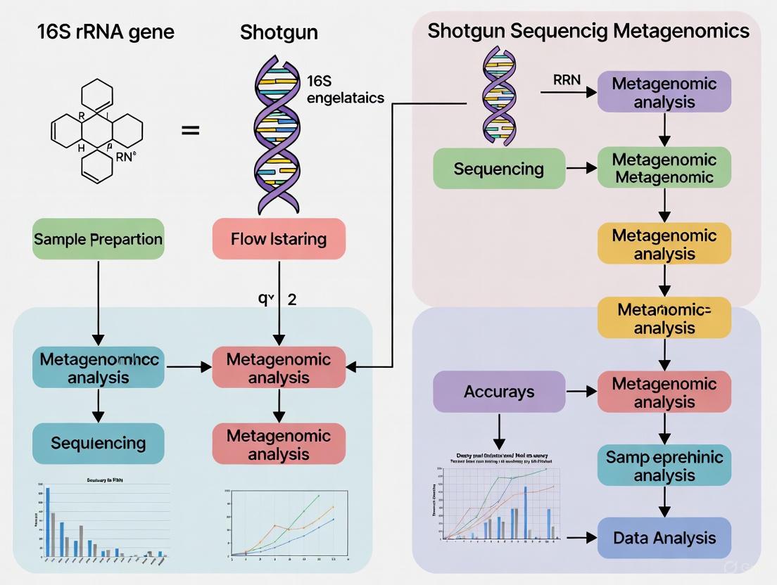
The following diagram illustrates the core workflow from sample to insight:

Shotgun Metagenomics vs. 16S rRNA Sequencing: A Detailed Comparison

For beginners, understanding the distinction between shotgun metagenomics and the more traditional 16S rRNA sequencing is critical for selecting the appropriate method. The table below summarizes the key differences.

Factor	16S rRNA Sequencing	Shotgun Metagenomic Sequencing
Principle	Targeted amplicon sequencing of the 16S rRNA gene [1]	Untargeted sequencing of all genomic DNA [1]
Taxonomic Resolution	Genus-level (sometimes species) [1] [15]	Species and strain-level resolution [1] [15]
Taxonomic Coverage	Bacteria and Archaea only [1]	All domains: Bacteria, Archaea, Viruses, Fungi, Protists [1] [12]
Functional Profiling	No direct functional data; only prediction via tools like PICRUSt [1] [15]	Yes, direct identification of functional genes and pathways [1] [15]
Cost per Sample	Lower (~$50-$80 USD) [1] [15]	Higher (~$150-$200 USD for deep sequencing) [1] [15]
Host DNA Interference	Low (PCR targets microbial gene) [12] [15]	High (sequences all DNA, requiring host depletion) [1] [15]
Bioinformatics	Less complex, established pipelines (e.g., QIIME, MOTHUR) [1]	More complex, requires greater computational power [11] [1]
Bias	Medium-High (primer choice, copy number variation) [1]	Lower (no PCR amplification step) [11] [1]
Recommended Sample Type	All, especially low-biomass/high-host-DNA samples [12] [15]	All, but optimal for high-microbial-biomass samples like stool [12] [15]

Choosing the Right Lens for Your Research

Comparative studies consistently show that shotgun sequencing provides a more detailed and powerful view of microbial communities. For example, one study found that when a sufficient number of reads is available, shotgun sequencing identifies a statistically significant higher number of less abundant taxa that 16S sequencing misses [13]. These less abundant genera are biologically meaningful and can discriminate between experimental conditions as effectively as more abundant genera [13].

Another study on the human gut microbiome concluded that while both methods can reveal common patterns, "shotgun often gives a more detailed snapshot than 16S, both in depth and breadth. Instead, 16S will tend to show only part of the picture, giving greater weight to dominant bacteria in a sample" [16].

Therefore, the choice depends on the research question, sample type, and available resources. Shotgun metagenomics is preferred for in-depth analyses of well-characterized environments (e.g., human gut) where strain-level resolution and functional potential are needed [16]. 16S rRNA sequencing remains a cost-effective option for large-scale studies focused solely on bacterial composition or when analyzing samples with high host DNA contamination, such as tissue biopsies [1] [16].

The Scientist's Toolkit: Essential Reagents and Solutions

Successful shotgun metagenomic sequencing relies on a suite of specialized reagents and tools.

Tool/Reagent	Function	Examples & Notes
DNA Extraction Kit	Lyses microbial cells and purifies genomic DNA from complex samples.	NucleoSpin Soil Kit, DNeasy PowerLyzer PowerSoil Kit [16]. Choice critical for bias minimization.
Fragmentation Enzymes	Randomly shears purified DNA into short fragments for library prep.	Tagmentation enzymes (e.g., Illumina Nextera) simplify the process [1].
Library Prep Kit	Prepares DNA for sequencing via end-repair, adapter ligation, and PCR amplification.	Illumina DNA Prep kits. Includes index adapters for sample multiplexing [11].
Sequencing Control	Validates entire workflow, from extraction to bioinformatics.	ZymoBIOMICS Microbial Community Standard (mock community with known composition) [15].
Bioinformatics Pipelines	Processes raw data for taxonomic and functional analysis.	Kraken2 (taxonomy), MetaPhlAn (marker genes), HUMAnN (function), MEGAHIT (assembly) [11] [14].
Reference Databases	Curated collections of genomes or genes for classifying sequencing reads.	NCBI RefSeq, GTDB, SILVA. Accuracy depends on database quality and completeness [11] [16].

Shotgun metagenomic sequencing represents a paradigm shift in microbiology, offering an unparalleled, comprehensive view of the genetic landscape of entire microbial ecosystems. By capturing all genetic material in a sample, it enables researchers to move beyond mere census-taking to understanding the functional capabilities that govern microbial life. While 16S rRNA sequencing retains its place for specific, targeted applications, shotgun metagenomics is the definitive tool for researchers and drug development professionals seeking a high-resolution, functional understanding of the microbiome in health, disease, and the environment.

The study of complex microbial communities has been revolutionized by high-throughput sequencing technologies. Two principal methods dominate this field: 16S rRNA gene sequencing and shotgun metagenomic sequencing [13] [12]. Each method offers distinct advantages and limitations, making the choice between them critical for research outcomes, especially in drug development and clinical diagnostics [1]. This guide provides an in-depth technical comparison of their core workflows, from initial sample preparation to final data output, framed for beginners and professionals embarking on microbiome research.

The fundamental distinction lies in their scope and approach. 16S rRNA sequencing is a targeted amplicon method that amplifies and sequences a specific, conserved genetic marker—the 16S ribosomal RNA gene—found in all bacteria and archaea [17] [18]. In contrast, shotgun metagenomics takes a comprehensive approach by randomly fragmenting and sequencing all the DNA present in a sample, enabling the reconstruction of entire genomes and providing access to the functional gene content of the community [13] [19].

Fundamental Methodological Differences

The choice between these methods fundamentally shapes the type and quality of information obtained. The table below summarizes their core characteristics.

Table 1: Core Characteristics of 16S rRNA and Shotgun Metagenomic Sequencing

Characteristic	16S rRNA Sequencing	Shotgun Metagenomic Sequencing
Methodology	Targeted PCR amplification of the 16S rRNA gene [17] [1]	Untargeted, random fragmentation and sequencing of all DNA [12] [19]
Primary Output	Sequencing reads of one or more hypervariable regions (V1-V9) [17]	Sequencing reads from across all genomic DNA in the sample [12]
Taxonomic Scope	Bacteria and Archaea only [12] [1]	All domains: Bacteria, Archaea, Viruses, Fungi, and Protists [18] [12]
Typical Taxonomic Resolution	Genus-level (species-level possible but can be unreliable) [18] [1]	Species-level and strain-level (including single nucleotide variants) [17] [1]
Functional Profiling	No direct assessment; requires prediction tools (e.g., PICRUSt) [17] [1]	Direct characterization of functional genes and metabolic pathways [18] [1]
Relative Cost per Sample	Lower (~$50 - $80 USD) [17] [1]	Higher, 2-3x that of 16S; ~$150-$200 USD for deep sequencing [17] [1]
Bioinformatics Complexity	Beginner to Intermediate [18] [1]	Intermediate to Advanced [18] [1]
Sensitivity to Host DNA	Low (PCR targets microbial gene) [17] [12]	High (sequences all DNA; host depletion may be needed) [17] [12]
Minimum DNA Input	Very low (can work with < 1 ng or 10 gene copies) [17] [12]	Higher (typically requires a minimum of 1 ng) [17] [12]

DNA Extraction and Quality Control

The journey for both workflows begins with the extraction of high-quality DNA from the sample, a step that profoundly impacts all downstream results [20] [21]. The goal is to obtain a representative and unbiased genomic DNA sample that accurately reflects the microbial community.

Critical Steps in DNA Extraction

Sample homogenization is crucial for subsampling representative microbial biomass [20]. Efficient cell lysis is paramount, particularly for breaking down the tough peptidoglycan cell walls of Gram-positive bacteria. The inclusion of a robust bead-beating step is now widely recommended to ensure their adequate lysis and to prevent underrepresentation [20] [21]. Finally, the purification process must effectively remove contaminants like proteins and enzymatic inhibitors that can interfere with subsequent library preparation and sequencing [22].

Comparison of Extraction Kits and Protocols

Recent studies have systematically compared commercial DNA extraction kits to identify best practices. One study evaluated four common methods—NucleoSpin Soil Kit (Macherey-Nagel, MN), DNeasy PowerLyzer PowerSoil Kit (QIAGEN, DQ), QIAamp Fast DNA Stool Kit (QIAGEN, QQ), and ZymoBIOMICS DNA Mini Kit (ZymoResearch, Z)—with and without a stool preprocessing device (SPD) [20]. Another independent evaluation compared kits from Qiagen (Q), Macherey-Nagel (MN), Invitrogen (I), and Zymo Research (Z) for gut microbiome studies [21].

Table 2: Comparison of DNA Extraction Kit Performance Based on Experimental Data

Extraction Kit / Protocol	DNA Yield	DNA Quality / Purity (A260/280)	Impact on Alpha-Diversity	Key Findings
SPD + DNeasy PowerLyzer (S-DQ)	High	Excellent (~1.8) [20]	High	Best overall performance; high yield, purity, and diversity [20]
ZymoBIOMICS (Z)	Low to Moderate [20]	Good [20]	High [20]	Most consistent results with minimal variation; suitable for long-read sequencing [21]
SPD + ZymoBIOMICS (S-Z)	High [20]	Good [20]	High [20]	High percentage of samples >5 ng/μL (88%) [20]
Macherey-Nagel (MN)	Highest yield in one study [21]	Moderate [20]	High [20]	High yield, but may require SPD for optimal results [20]
Qiagen (Q)	Low [21]	Low (degraded DNA) [21]	Not Reported	Highest host DNA ratio; not recommended for samples with high host contamination [21]

Library Preparation and Sequencing

Following DNA extraction, the paths of the two methods diverge significantly during library preparation—the process of converting purified DNA into a format compatible with the sequencing platform.

16S rRNA Sequencing Workflow

The 16S workflow is a PCR-dependent, targeted approach [17] [1]. It begins with the selection of universal primers that bind to conserved regions flanking one or more of the nine hypervariable regions (V1-V9) of the 16S rRNA gene. The choice of which variable region(s) to amplify can introduce bias, as different primers have varying coverage and efficiency for different bacterial taxa [13] [22]. The targeted regions are then amplified via polymerase chain reaction (PCR). During this step, sample-specific molecular barcodes (indexes) are added to the amplicons, allowing multiple samples to be pooled and sequenced simultaneously in a single run—a process known as multiplexing [17] [1]. The final library is a pool of these barcoded amplicons, which is then quantified and normalized before loading onto a sequencer. The Illumina MiSeq platform is commonly used for 16S sequencing due to its optimized output and read lengths for amplicon studies [19].

Shotgun Metagenomic Sequencing Workflow

The shotgun metagenomics workflow is PCR-free in its core sequencing step and aims to be untargeted [12] [19]. The extracted genomic DNA is first randomly fragmented. This can be achieved through physical (e.g., acoustic shearing) or enzymatic methods (e.g., tagmentation) [1] [19]. Adapter sequences, which are essential for binding to the sequencing flow cell and initiating the sequencing reaction, are then ligated to the fragmented DNA. Like the 16S workflow, sample-specific barcodes are incorporated during a subsequent PCR amplification step that also enriches for adapter-ligated fragments. The final library is a complex mixture of fragments representing the entire genetic material of the sample. Given the vast complexity and to achieve sufficient coverage of microbial genomes, shotgun metagenomics typically requires a much higher sequencing depth (more reads per sample) than 16S sequencing, making it more expensive, though "shallow shotgun" approaches offer a cost-compromise for certain study designs [12] [1].

Data Analysis and Bioinformatics

The data analysis pipelines for 16S and shotgun sequencing are fundamentally different, reflecting the nature of the raw data generated.

16S rRNA Data Analysis Pipeline

The goal of 16S data analysis is to convert raw sequencing reads into a taxonomic profile of the bacterial community [22]. The process typically involves:

• Quality Filtering and Trimming: Raw sequences are processed to remove low-quality bases, adapter sequences, and primers [22].
• Denoising and Clustering: High-quality sequences are then either clustered into Operational Taxonomic Units (OTUs) based on a sequence similarity threshold (e.g., 97%) or resolved into Amplicon Sequence Variants (ASVs) using error-correction algorithms like DADA2. ASVs offer higher resolution by distinguishing single-nucleotide differences [21] [1].
• Taxonomic Assignment: The resulting OTUs or ASVs are compared against curated 16S reference databases (e.g., SILVA, Greengenes, RDP) to assign taxonomic classifications from phylum to genus or species [18] [22].
• Downstream Analysis: The final output is a feature table (counts of OTUs/ASVs per sample) which is used for ecological analyses like alpha-diversity (within-sample diversity) and beta-diversity (between-sample diversity), and statistical comparisons between sample groups [22].

Shotgun Metagenomic Data Analysis Pipeline

Shotgun data analysis is more complex and computationally intensive, but it provides both taxonomic and functional insights [23] [19]. Two primary analytical strategies are employed:

• Read-Based Taxonomy Profiling: In this assembly-free approach, individual sequencing reads are directly aligned to comprehensive genomic databases (e.g., RefSeq) using tools like Kraken2 or MetaPhlAn to determine "who is there" at a high taxonomic resolution [21] [19].
• Assembly-Based Analysis: For a more in-depth view, reads can be assembled into longer contiguous sequences (contigs). This is one of the most computationally challenging steps in bioinformatics [23]. The assembled contigs are then binned into putative genomes (Metagenome-Assembled Genomes, MAGs). These MAGs can be annotated to identify open reading frames (ORFs) and predict genes. The predicted genes are then functionally annotated by comparing them to databases like KEGG, COG, and CAZy to understand "what they are doing" in terms of metabolic pathways, virulence factors, and antibiotic resistance genes [22] [19].

The Scientist's Toolkit: Essential Reagents and Software

Successful execution of a metagenomic study relies on a suite of trusted laboratory reagents and bioinformatics tools.

Table 3: Essential Research Reagents and Bioinformatics Tools

Category	Item	Function / Application
DNA Extraction Kits	DNeasy PowerLyzer PowerSoil (QIAGEN) [20]	Efficient lysis of diverse bacteria, including Gram-positives; high DNA yield and purity.
	ZymoBIOMICS DNA Miniprep (Zymo Research) [20] [21]	Consistent performance and high-quality DNA suitable for long-read sequencing.
Library Prep Kits	Illumina DNA Prep [21]	Library preparation for shotgun metagenomic sequencing on Illumina platforms.
	Various 16S Amplicon Kits (e.g., Zymo) [21]	PCR amplification and barcoding of specific 16S rRNA hypervariable regions.
Bioinformatics Tools (16S)	QIIME2, MOTHUR [18] [1]	Integrated pipelines for 16S data analysis from quality filtering to diversity analysis.
	DADA2 [21] [1]	Error-correction algorithm for resolving Amplicon Sequence Variants (ASVs).
Bioinformatics Tools (Shotgun)	Kraken2 [21] [19]	Fast and accurate taxonomic classification of shotgun sequencing reads.
	MetaPhlAn [17] [1]	Profiler of microbial composition using unique clade-specific marker genes.
	HUMAnN [1] [19]	Pipeline for quantifying the abundance of microbial metabolic pathways.
	MEGAHIT, metaSPAdes [1] [19]	Efficient and sensitive de novo assemblers for metagenomic data.
Reference Databases (16S)	SILVA, Greengenes, RDP [18] [22]	Curated databases of 16S rRNA sequences for taxonomic assignment.
Reference Databases (Shotgun)	KEGG, COG, eggNOG [19]	Databases for functional annotation of genes and pathways.
	CARD [19]	Comprehensive Antibiotic Resistance Database for annotating AMR genes.
	RefSeq [21] [19]	Comprehensive genome database for taxonomic profiling.

The choice between 16S rRNA gene sequencing and shotgun metagenomic sequencing is not a matter of one being universally superior to the other, but rather of selecting the right tool for the specific research question, budget, and analytical capabilities [12] [1].

16S rRNA sequencing remains a powerful, cost-effective method for large-scale studies focused primarily on the taxonomic composition of bacterial and archaeal communities, especially when the research involves hundreds or thousands of samples or when dealing with low-biomass samples where host DNA contamination is a concern [17] [12].

Shotgun metagenomic sequencing is the necessary choice when the research objectives require high-resolution taxonomic profiling (to the species or strain level), the detection of non-bacterial kingdom members (viruses, fungi), or direct insight into the functional potential of the microbiome, such as identifying antibiotic resistance genes or metabolic pathways relevant to drug development and host-health interactions [18] [1].

For researchers beginning a project, the decision matrix should carefully balance the need for resolution and functional data against constraints of budget, sample type, and bioinformatics resources. As sequencing costs continue to fall and analytical tools become more user-friendly, shotgun metagenomics is becoming increasingly accessible, promising a deeper and more comprehensive understanding of the microbial world in the years to come [19].

For researchers embarking on the study of microbial communities, navigating the terminology and methodology choices between 16S rRNA gene sequencing and shotgun metagenomics is a critical first step. The selection between these approaches fundamentally shapes the resolution of taxonomic data, the depth of functional insights, and the overall interpretation of microbiome study results. This guide demystifies four essential concepts—Reads, OTUs, ASVs, and Taxonomic Resolution—within the practical context of choosing between 16S rRNA and shotgun metagenomic sequencing, providing a foundation for making informed decisions in experimental design.

Core Terminology Defined

Reads

Reads are the fundamental strings of DNA sequence output by sequencing instruments [24]. In the context of microbiome studies, they represent short fragments of genetic material that are later pieced together or classified to determine what organisms are present in a sample.

• In 16S rRNA Sequencing: Reads originate from a specific, targeted region of the 16S rRNA gene that has been amplified by PCR. The number of reads corresponding to a particular organism is used to estimate its relative abundance in the microbial community [24] [25].
• In Shotgun Metagenomic Sequencing: Reads are generated from random fragments of all genomic DNA present in a sample (including bacteria, archaea, viruses, fungi, and host DNA). This allows for a broader survey of the community but typically requires a much higher number of reads per sample to achieve sufficient coverage for accurate taxonomic and functional analysis [13] [26].

OTUs (Operational Taxonomic Units)

OTUs are clusters of similar sequencing reads, traditionally grouped based on a percent sequence similarity threshold, most commonly 97%, which is intended to approximate bacterial species-level differences [27] [28].

• Methodology: Reads are clustered together into bins or "units" if they are at least 97% identical. This process groups closely related sequences, smoothing out minor variations often caused by sequencing errors [27].
• Key Characteristics:
  • Resolution: Lower resolution compared to ASVs, as genetically distinct but closely related sequences may be grouped [27].
  • Error Handling: Tolerates sequencing errors by absorbing them into clusters [27] [28].
  • Computational Demand: Generally less computationally intensive than ASV methods [27].

ASVs (Amplicon Sequence Variants)

ASVs are unique, error-corrected DNA sequences that represent exact biological sequences present in a sample, providing single-nucleotide resolution [27] [28].

• Methodology: Instead of clustering, ASV methods (e.g., DADA2) use a denoising algorithm to distinguish true biological variation from sequencing errors. This results in a table of unique sequences without arbitrary clustering thresholds [27] [26].
• Key Characteristics:
  • Resolution: High-resolution, capable of distinguishing closely related microbial strains [27] [29].
  • Error Handling: Actively models and removes sequencing errors, leading to higher accuracy [27] [28].
  • Reproducibility: ASVs are exact sequences, making them highly reproducible and comparable across different studies [27].

Table 1: Head-to-Head Comparison of OTUs and ASVs

Feature	OTUs (Operational Taxonomic Units)	ASVs (Amplicon Sequence Variants)
Definition	Clusters of sequences with a defined similarity threshold (e.g., 97%)	Exact, error-corrected sequence variants
Resolution	Lower (cluster-level)	Higher (single-nucleotide)
Error Handling	Errors can be absorbed into clusters	Uses algorithms to denoise and correct errors
Reproducibility	May vary between studies and parameters	Highly reproducible across studies
Computational Cost	Less demanding	More demanding due to denoising
Primary Advantage	Computational efficiency, error tolerance	Precision, reproducibility, fine-scale differentiation

Taxonomic Resolution

Taxonomic Resolution refers to the level of taxonomic classification (e.g., phylum, family, genus, species, or strain) that can be reliably assigned from sequencing data [1]. The choice between 16S rRNA and shotgun sequencing is a primary determinant of the achievable resolution.

• 16S rRNA Sequencing: Typically provides reliable identification down to the genus level, and sometimes to the species level, depending on the hypervariable region targeted and the bioinformatics tool used [1] [29]. However, its reliance on a single gene and the high conservation of the 16S rRNA gene limit its ability to differentiate between closely related species or strains [30].
• Shotgun Metagenomic Sequencing: By utilizing information from the entire genome, shotgun sequencing can achieve species-level and often strain-level resolution [13] [1] [30]. This allows researchers to investigate functional capabilities and track specific strains within a microbial community.

Diagram 1: Bioinformatic Paths from Reads to Taxonomy. This workflow illustrates the two primary methods for processing 16S rRNA sequencing reads and their impact on the final taxonomic resolution.

16S rRNA vs. Shotgun Metagenomic Sequencing: A Practical Comparison

The choice between 16S and shotgun sequencing involves balancing cost, depth of information, and technical requirements. The following table and experimental overview highlight the key differences to inform this decision.

Table 2: 16S rRNA Sequencing vs. Shotgun Metagenomic Sequencing

Factor	16S rRNA Sequencing	Shotgun Metagenomic Sequencing
Cost (per sample)	~$50 - $80 [1] [29]	Starting at ~$150 - $200 [1] [29]
Target	Amplified 16S rRNA gene regions	All genomic DNA in a sample
Taxonomic Resolution	Genus-level (sometimes species) [1] [30]	Species-level and strain-level [13] [1]
Taxonomic Coverage	Bacteria and Archaea only [1] [25]	All domains (Bacteria, Archaea, Fungi, Viruses) [1] [26]
Functional Profiling	No (only predicted via tools like PICRUSt) [1] [30]	Yes (direct assessment of genes and pathways) [1] [29]
Host DNA Interference	Low (due to targeted PCR) [29]	High (can be a major issue in non-fecal samples) [1] [29]
Bioinformatics Complexity	Beginner to Intermediate [1]	Intermediate to Advanced [1]
Recommended Sample Type	All sample types, including low-biomass [1] [29]	Best for samples with low host DNA (e.g., feces) [29]

16S rRNA Gene Sequencing Workflow [24] [25]:

• DNA Extraction: Isolate genomic DNA from the sample (e.g., soil, stool, water).
• PCR Amplification: Use primers targeting specific hypervariable regions (e.g., V3-V4) of the 16S rRNA gene to amplify the target.
• Library Preparation: Clean the PCR products and attach molecular barcodes (indexes) to pool multiple samples.
• Sequencing: Sequence the pooled library on a platform like Illumina MiSeq.
• Bioinformatic Analysis:
  • Quality Filtering: Remove low-quality reads and sequencing errors.
  • OTU/ASV Generation: Cluster reads into OTUs (e.g., using QIIME) or infer ASVs (e.g., using DADA2).
  • Taxonomic Assignment: Assign taxonomy by comparing OTUs/ASVs to reference databases (e.g., SILVA, Greengenes).

Shotgun Metagenomic Sequencing Workflow [1] [30]:

• DNA Extraction: Isolate total genomic DNA from the sample.
• Library Preparation: Fragment the DNA, often via tagmentation, and ligate adapter sequences without target-specific amplification.
• Sequencing: Sequence the entire library on a platform like Illumina HiSeq or NovaSeq to generate tens of millions of reads per sample.
• Bioinformatic Analysis:
  • Quality Control & Host Filtering: Trim reads and remove sequences originating from the host (e.g., human) genome.
  • Taxonomic Profiling: Assign reads to taxa using marker-based (e.g., MetaPhlAn) or k-mer-based (e.g., Kraken2) tools.
  • Functional Profiling: Map reads to functional databases (e.g., KEGG, eggNOG) to determine gene and pathway abundances.
  • Advanced Option - Genome-Resolved Metagenomics: Assemble reads into longer contigs and bin them into Metagenome-Assembled Genomes (MAGs), which can represent novel, uncultured microbes [30].

Diagram 2: Comparative Workflows for Microbiome Sequencing. This diagram contrasts the targeted approach of 16S rRNA sequencing with the comprehensive, untargeted approach of shotgun metagenomics, which can be extended to genome-resolved analysis (MAGs).

The Scientist's Toolkit: Essential Reagents and Materials

Successful microbiome sequencing relies on a suite of specialized reagents and kits. The following table details key solutions for major experimental steps.

Table 3: Research Reagent Solutions for Microbiome Sequencing

Item	Function	Examples & Notes
Sample Preservation Kits	Stabilizes microbial community at collection to prevent shifts in composition before DNA extraction.	OMR-200 tubes (OMNIgene GUT) [26]. Critical for field work and clinical sampling.
DNA Extraction Kits	Lyse microbial cells and purify genomic DNA from complex sample matrices (e.g., stool, soil).	Kits from Mo Bio (now Qiagen), Zymo Research [25]. Choice of kit can impact yield and community representation.
PCR Enzymes & Primers	For 16S sequencing: Amplify target hypervariable regions with high fidelity and minimal bias.	PrimeSTAR GXL DNA Polymerase, 16S V4 primer set (515F/806R) [24] [25].
Library Preparation Kits	Prepare sequencing libraries from either PCR amplicons (16S) or fragmented genomic DNA (shotgun).	Illumina Nextera XT DNA Library Preparation Kit [1].
Mock Microbial Communities	Serve as positive controls containing known, predefined mixes of microbial cells or DNA to validate the entire workflow.	ZymoBIOMICS Microbial Community Standard [28] [29]. Essential for benchmarking performance.
Host DNA Depletion Kits	Selectively remove host (e.g., human) DNA from samples to increase the proportion of microbial reads in shotgun sequencing.	HostZERO Microbial DNA Kit [29]. Particularly useful for tissue and blood samples.

Key Experimental Findings and Data Interpretation

Detection Power and Taxonomic Profiles

A direct comparison study on chicken gut microbiota revealed that shotgun sequencing, when performed at sufficient depth (>500,000 reads per sample), identifies a statistically significant higher number of taxa compared to 16S sequencing [13]. The additional taxa detected by shotgun are typically low-abundance genera, which were shown to be biologically meaningful and capable of discriminating between experimental conditions (e.g., different GI tract compartments) as effectively as the more abundant genera [13]. Furthermore, shotgun sequencing identified 152 statistically significant changes in genera abundance between gut compartments that 16S sequencing failed to detect [13].

The "Goldilocks" Effect in Taxonomic Resolution

In a machine learning study aimed at classifying colorectal cancer from microbiome data, model performance increased with finer taxonomic resolution—but only up to a point. Performance peaked at the family, genus, and OTU levels before significantly decreasing at the ASV level [31]. This suggests that while coarse resolution (e.g., phylum) lacks distinctness, very fine resolution (ASV) can be overly individualized and sparse, hindering classification. For certain predictive applications, mid-range resolution (genus/OTU) is "just right" [31].

Concordance and Discordance in Abundance Measures

Despite different approaches, 16S and shotgun sequencing often show good agreement in quantifying common taxa. A study on infant gut microbiomes reported an average correlation of 0.69 for genus-level abundances between the two methods [13]. However, discrepancies arise, often related to the detection limits of 16S sequencing, where it partially or completely misses genera that are identified by the more sensitive shotgun approach [13].

Strategic Application: Matching Your Research Goals to the Right Tool

Taxonomic profiling is a fundamental step in microbiome research, enabling scientists to answer the critical question: "Who is there?" in a complex microbial community. The choice of sequencing method directly determines the resolution of the answer, fundamentally shaping the biological insights that can be gained. For researchers, scientists, and drug development professionals entering the field, understanding the distinction between 16S rRNA gene sequencing and shotgun metagenomic sequencing is crucial for appropriate experimental design and data interpretation. While 16S rRNA sequencing provides a cost-effective overview primarily at the genus level, shotgun metagenomics unlocks species- and strain-level resolution along with functional potential, albeit at a higher cost and computational burden [1] [6]. This technical guide provides an in-depth comparison of these two cornerstone methods, focusing on their taxonomic resolution, supported by quantitative data, detailed experimental protocols, and essential bioinformatic considerations to inform your research strategy.

Core Principles and Technical Comparisons

16S rRNA Gene Sequencing (Metataxonomics)

The 16S rRNA gene is a highly conserved component of the prokaryotic ribosome, containing nine hypervariable regions (V1-V9) that provide phylogenetic signatures for taxonomic assignment [32] [16]. 16S rRNA gene sequencing is a form of amplicon sequencing that uses polymerase chain reaction (PCR) to amplify one or more of these hypervariable regions before sequencing [1] [33]. The process begins with DNA extraction, followed by a critical primer selection step where researchers choose specific primers to target hypervariable regions (e.g., V3-V4 for bacterial general profiling) [32] [16]. The PCR amplification step introduces primers with molecular barcodes to allow sample multiplexing, after which the amplified DNA is cleaned, quantified, and sequenced [1]. Bioinformatic processing then involves quality filtering, clustering of sequences into Operational Taxonomic Units (OTUs) or denoising into Amplicon Sequence Variants (ASVs), and finally taxonomic classification by comparing these clusters to reference databases such as SILVA or Greengenes [1] [16].

A key limitation of this method is its resolution ceiling. Due to the conservation and length of the sequenced gene fragment, 16S rRNA sequencing is generally reliable for taxonomic assignment at the genus level, with species-level identification often being unreliable and strain-level differentiation impossible [1] [33] [12]. Furthermore, as it targets a gene unique to bacteria and archaea, it cannot profile other microbial domains like fungi, viruses, or protists without additional, targeted approaches (e.g., ITS sequencing for fungi) [1] [32].

Shotgun Metagenomic Sequencing

In contrast, shotgun metagenomic sequencing takes an untargeted approach by sequencing all the DNA fragments present in a sample [1] [32]. The process begins with DNA extraction, but instead of targeted PCR amplification, the extracted DNA is randomly fragmented (a process often involving tagmentation) and prepared for sequencing with the addition of adapters and barcodes [1] [6]. These fragments are then sequenced at high depth. Because the entire genetic content is sequenced, the resulting data can be aligned to comprehensive genomic databases. Taxonomic profiling is achieved using tools like MetaPhlAn (which uses marker genes) or Kraken2 (which uses k-mer matching) that compare the short reads to entire microbial genomes in databases such as the NCBI RefSeq Genome Database [1] [33]. This allows for identification and profiling of all domains of life—bacteria, archaea, fungi, viruses, and protists—simultaneously from a single library preparation [12] [6].

The primary advantage of shotgun sequencing is its superior taxonomic resolution. By accessing the entire genomic content rather than a single gene, it reliably achieves species-level identification and can often discriminate between different strains of the same species by profiling single nucleotide variants (SNVs), provided the sequencing depth is sufficient [1] [33].

Side-by-Side Technical Comparison

Table 1: Core Technical Comparison of 16S rRNA and Shotgun Metagenomic Sequencing

Factor	16S rRNA Sequencing	Shotgun Metagenomic Sequencing
Target	Specific hypervariable regions of the 16S rRNA gene [1] [32]	All genomic DNA in a sample [1] [6]
Taxonomic Resolution	Genus-level (sometimes species-level) [1] [33]	Species-level and often strain-level [1] [33]
Taxonomic Coverage	Bacteria and Archaea only [1] [12]	All domains: Bacteria, Archaea, Fungi, Viruses, Protists [1] [12]
Functional Profiling	No direct functional data; only prediction via tools like PICRUSt [1] [33]	Yes, direct profiling of microbial genes and metabolic pathways [1] [33]
Cost per Sample (USD)	~$50 - $80 [1] [33]	~$150 - $200 (Standard); ~$120 (Shallow) [1] [33]
Minimum DNA Input	Very low (can work with <1 ng or 10 copies of the 16S gene) [33] [12]	Higher (typically requires a minimum of 1 ng) [33] [12]
Host DNA Interference	Low (PCR targets microbial gene specifically) [1] [33]	High (can be mitigated by host DNA depletion or increased sequencing depth) [1] [33]
Bioinformatics Complexity	Beginner to Intermediate [1]	Intermediate to Advanced [1]

Workflow Visualization

Quantitative Data and Performance Comparison

Empirical studies directly comparing the two methods consistently demonstrate that shotgun metagenomics provides a more powerful and detailed view of microbial communities, particularly for less abundant taxa.

Detection Power and Abundance Correlation

A seminal study on the chicken gut microbiota provided stark evidence of the difference in detection power. When comparing genera abundance between two gastrointestinal compartments (caeca vs. crop), shotgun sequencing identified 256 statistically significant differences, whereas 16S sequencing identified only 108 [13]. Notably, shotgun sequencing found 152 significant changes that 16S missed, while 16S found only 4 unique significant changes [13]. This indicates that the additional taxa detected by shotgun are not just present but biologically meaningful and responsive to experimental conditions.

Furthermore, a 2024 study on human colorectal cancer compared 156 stool samples sequenced with both techniques. It confirmed that 16S sequencing detects only part of the gut microbiota community revealed by shotgun sequencing, with a tendency to show greater weight to dominant bacteria [16]. Despite this, the abundance of taxa common to both methods is generally positively correlated. Research in infant gut microbiomes has shown a good agreement between the techniques for shared genera, with an average Pearson’s correlation coefficient of 0.69 ± 0.03 in one analysis [13] [26].

Resolution and Diversity Metrics

The same 2024 study also highlighted differences in data structure. At the genus level, the relative species abundance (RSA) distributions from shotgun sequencing were more symmetrical (skewness closer to zero), whereas distributions from 16S were more left-skewed, a pattern often indicative of a smaller effective sample size and the truncation of rare taxa [13] [16]. Shotgun sequencing typically results in higher observed alpha diversity (within-sample diversity) because it can detect a greater number of rare species [16]. While both methods can reveal similar beta-diversity (between-sample diversity) patterns in studies of strong effect sizes, the additional detail from shotgun data provides more power to distinguish between subtle community differences [1] [16].

Table 2: Empirical Performance Comparison from Peer-Reviewed Studies

Performance Metric	16S rRNA Sequencing	Shotgun Metagenomic Sequencing	Research Context
Significant Genera Differences	108 [13]	256 [13]	Chicken GI Tract Compartments [13]
Sparsity of Data	Higher [16]	Lower [16]	Human Colorectal Cancer [16]
Alpha Diversity	Lower observed diversity [16]	Higher observed diversity [16]	Human Colorectal Cancer [16]
Correlation of Abundances	0.69 ± 0.03 (for shared genera) [13]	0.69 ± 0.03 (for shared genera) [13]	Chicken GI Tract [13]
Strain-Level Resolution	Not achievable [1]	Possible by profiling single nucleotide variants [1]	General Microbiome Research [1]

Detailed Experimental Protocols

To ensure reproducible results, the following core protocols detail the key steps for both sequencing methods.

Protocol for 16S rRNA Gene Sequencing

This protocol is adapted from standard procedures used in recent literature [1] [32] [16].

• DNA Extraction: Extract genomic DNA from the sample (e.g., stool, soil, swab) using a dedicated kit such as the DNeasy PowerLyzer PowerSoil kit (Qiagen) or NucleoSpin Soil Kit (Macherey-Nagel). The choice of kit can impact yield and should be consistent within a study [34] [16].
• PCR Amplification: Amplify the target hypervariable region(s) (e.g., V3-V4) using primers fused with Illumina adapter sequences and sample-specific barcodes. Use a high-fidelity polymerase to minimize PCR errors. The number of PCR cycles should be optimized to avoid over-amplification [32] [16].
• Clean-up and Normalization: Purify the PCR amplicons to remove enzymes, primers, and other impurities. Methods include bead-based cleanups (e.g., AMPure XP beads) or column-based purification. Quantify the DNA and pool the barcoded samples in equimolar amounts [1] [34].
• Library Quantification and Sequencing: Precisely quantify the final pooled library using methods such as fluorometry (Qubit) or quantitative PCR (qPCR). Load the pool onto a sequencer, such as an Illumina MiSeq, which is commonly used for amplicon studies due to its read length and output [1] [32].

Protocol for Shotgun Metagenomic Sequencing

This protocol outlines the steps for whole-genome shotgun sequencing, commonly used in human gut microbiome studies [1] [32] [16].

• DNA Extraction and QC: Extract high-quality, high-molecular-weight DNA. For samples with high host DNA content (e.g., tissue, blood), consider using a host depletion kit. Quantify the DNA using a fluorometer and assess fragment size distribution with an automated electrophoresis system (e.g., LabChip GX) [34] [16].
• Library Preparation (Tagmentation): Fragment the purified DNA and ligate sequencing adapters. This is often done in a single-step "tagmentation" reaction using kits like the Nextera DNA Flex (Illumina). This step also indexes the samples with unique dual indices (UDIs) for multiplexing [1] [34].
• Library Amplification and Clean-up: Perform a limited-cycle PCR to amplify the tagmented libraries. Clean up the final libraries to remove PCR constituents and select for the appropriate fragment size using bead-based size selection [1].
• Pooling, QC, and Sequencing: Quantify the final libraries, pool them in equimolar ratios, and perform rigorous QC. Sequence the pool on a high-output platform like the Illumina NovaSeq or HiSeq to achieve the millions of reads per sample required for sufficient microbial coverage [1] [34].

The Scientist's Toolkit: Essential Research Reagents

The following reagents and kits are fundamental to executing the protocols described above and generating high-quality data.

Table 3: Key Research Reagent Solutions for Metagenomic Sequencing

Reagent/Kits	Function	Example Products
Microbial DNA Extraction Kits	Isolate pure, inhibitor-free genomic DNA from complex samples.	NucleoSpin Soil Kit (Macherey-Nagel), DNeasy PowerLyzer PowerSoil Kit (Qiagen) [34] [16]
16S rRNA PCR Primers & Kits	Amplify specific hypervariable regions of the 16S gene for sequencing.	Illumina 16S Metagenomic Sequencing Library Prep, custom V3-V4 primers (e.g., 341F/805R) [34] [32]
Shotgun Library Prep Kits	Fragment DNA, add adapters, and index samples for whole-genome sequencing.	Nextera DNA Flex Library Prep Kit (Illumina), NEXTFLEX Rapid XP V2 DNA-seq kit [34] [33]
Host DNA Depletion Kits	Remove host (e.g., human) DNA from samples to enrich for microbial signal.	HostZERO Microbial DNA Kit [33]
Library Quantification Kits	Accurately quantify sequencing libraries prior to pooling and loading.	Qubit dsDNA HS Assay Kit, Kapa Library Quantification Kit [34]
Bioinformatics Pipelines	Process raw sequencing data, perform quality control, and assign taxonomy.	16S: QIIME 2, DADA2, MOTHURShotgun: MetaPhlAn, Kraken2, HUMAnN [1] [33] [16]

The choice between 16S rRNA and shotgun metagenomic sequencing is a fundamental decision that dictates the scope and depth of a microbiome study. 16S rRNA sequencing is a powerful, cost-effective tool for large-scale ecological studies where the primary goal is to compare the relative composition of bacterial communities at the genus level across hundreds or thousands of samples [1] [26]. It is particularly suitable for samples with low microbial biomass or high host DNA content, such as skin swabs or tissue biopsies, where its targeted PCR approach is advantageous [1] [33].

Conversely, shotgun metagenomic sequencing is the necessary choice when the research demands the highest taxonomic resolution (species- and strain-level), comprehensive coverage of all microbial domains, or direct insight into the functional potential of the community [1] [16] [6]. It is highly recommended for stool samples, where microbial density is high, and for studies aiming to link specific microbes or their genes to host phenotypes, disease states, or drug responses [33] [16] [6].

For researchers designing new studies, a hybrid strategy is also emerging: using 16S sequencing for broad screening of a large sample set, followed by the selection of a critical subset of samples for deep shotgun sequencing. Furthermore, shallow shotgun sequencing presents a compelling intermediate option, offering much of the taxonomic and functional profiling power of deep shotgun at a cost closer to 16S sequencing, making it ideal for large cohort studies with well-characterized sample types like human feces [1] [12]. By aligning the technical capabilities of each method with the specific biological questions at hand, researchers can optimize resources and maximize the insights gained from their microbiome data.

Understanding the functional capabilities of a microbial community is essential for elucidating its role in human health, disease, and ecosystem functioning. For researchers beginning in microbiome science, two primary methods are used to gain these functional insights: shotgun metagenomic sequencing, which directly sequences all the genetic material in a sample, and 16S rRNA gene sequencing coupled with functional prediction tools like PICRUSt2 (Phylogenetic Investigation of Communities by Reconstruction of Unobserved States). The former provides direct measurement of genes but at higher cost and complexity, while the latter offers a cost-effective prediction based on taxonomic data, though with important limitations [10] [35] [36]. This technical guide provides an in-depth comparison of these approaches, framed within the context of 16S rRNA versus shotgun metagenomics for beginner researchers, drug development professionals, and scientists seeking to implement these methods in their work.

Core Methodologies and Fundamental Differences

Shotgun Metagenomic Sequencing: Direct Genetic Measurement

Shotgun metagenomic sequencing involves comprehensively sequencing all genes in all organisms present in a complex sample without targeting specific genetic regions [10]. This approach involves extracting total DNA from a sample, mechanically shearing it into small fragments (typically 250-300 bp), preparing sequencing libraries from these fragments, and sequencing them using next-generation sequencing platforms such as Illumina NovaSeq [35]. The resulting sequences provide a direct snapshot of the genetic potential of the entire microbial community, enabling researchers to identify which genes are present and their relative abundances. A key advantage of this method is its ability to simultaneously detect bacteria, archaea, fungi, viruses, and other microorganisms without prior targeting [36]. However, this method generates enormous datasets that require substantial computational resources for analysis, and can be complicated by host DNA contamination in samples like tissue biopsies [37] [38].

PICRUSt2: Predicting Function from 16S rRNA Data

PICRUSt2 is a bioinformatics tool that predicts the functional potential of a bacterial community based on 16S rRNA marker gene sequences [37] [39]. Unlike shotgun sequencing, it does not directly measure functional genes but infers them through a sophisticated phylogenetic placement algorithm. The methodology involves several key steps: first, 16S rRNA sequences are placed into a reference phylogeny containing 20,000 full-length 16S genes from bacterial and archaeal genomes; next, hidden state prediction algorithms infer gene family copy numbers for each amplicon sequence variant (ASV) based on the genomic content of phylogenetically related reference organisms; finally, these predictions are corrected for 16S rRNA copy number and multiplied by ASV abundances to generate a predicted metagenome [39] [40]. This approach leverages the rapidly growing number of sequenced microbial genomes (41,926 in PICRUSt2's default database) to make inferences about uncharacterized taxa [39].

Figure 1: The PICRUSt2 prediction workflow transforms 16S rRNA sequence data into functional predictions through phylogenetic placement and hidden state inference.

Critical Performance Comparison and Limitations

Accuracy Across Sample Types and Environments

Multiple benchmarking studies have revealed significant differences in how well functional prediction tools perform across different sample types. The performance of PICRUSt2 and similar tools is highly dependent on how well the microbial communities in a sample are represented in reference databases.

Table 1: Performance of Functional Prediction Tools Across Environments

Environment	Correlation with Shotgun Data	Inference Accuracy	Key Limitations
Human Gut	High (Spearman ρ: 0.79-0.88) [39]	Reasonable for inference [41]	Better for "housekeeping" functions [41]
Non-Human Primates	Moderate (Spearman ρ: ~0.79) [39]	Sharp degradation [41]	36.9% of predicted genes undetected by metagenomics [41]
Soil	Variable	Poor inference performance [41]	Underestimates specialized metabolic pathways [42]
Chicken Gut	Not specified	Not specified	39.5% of predicted genes undetected by metagenomics [41]

A critical finding from validation studies is that simple correlation coefficients between predicted and actual metagenomes can be misleading. Strong Spearman correlations (0.53-0.87) have been observed between PICRUSt2 predictions and shotgun metagenomes, but these strong correlations persist even when gene abundances are permuted across samples [41]. This indicates that correlation alone is an unreliable measure of prediction accuracy, as it may primarily reflect the underlying phylogenetic structure rather than true functional prediction power.

Performance Across Functional Categories

The accuracy of functional prediction tools varies substantially across different functional categories, with better performance for evolutionarily conserved "housekeeping" functions compared to specialized metabolic pathways.

Table 2: PICRUSt2 Performance by Functional Category Based on Human Gut Samples

Functional Category	Prediction Accuracy	Notes
Genetic Information Processing	Higher accuracy	Replication, repair, translation, folding, sorting, degradation [41]
Central Metabolism	Higher accuracy	Core metabolic functions [41]
Specialized Metabolism	Lower accuracy	Pathways with high phylogenetic variability [42]
Nitrogen & Carbon Cycling	Significant underestimation	Particularly problematic in environmental samples [42]

In soil environments, PICRUSt2 and Tax4Fun2 both show significant underestimation of gene frequencies in many KEGG categories, including genes with biogeochemical significance for soil carbon and nitrogen cycling [42]. PICRUSt2 functional profiles tend to represent greater relative abundances of genes in pathways for oxidative phosphorylation, while Tax4Fun2 detects more genes from specialized metabolic pathways, such as methane metabolism [42].

Experimental Protocols and Implementation

Shotgun Metagenomics Workflow

The standard workflow for shotgun metagenomic sequencing involves: (1) sample preparation with careful attention to minimizing host contamination; (2) DNA extraction using methods appropriate for the sample type (e.g., PowerSoil DNA Isolation kit for soil samples); (3) DNA fragmentation into 250-300 bp fragments; (4) library construction with 350bp insert size; (5) sequencing on platforms such as Illumina NovaSeq with paired-end 150 bp strategy; (6) bioinformatic processing including quality control to remove adapter sequences, unknown bases, and low-quality reads [35]. Downstream analysis typically involves taxonomic classification, gene prediction, functional annotation, and comparative analyses such as PCA and NMDS [35].

PICRUSt2 Analysis Pipeline

For PICRUSt2 analysis, the typical workflow involves: (1) obtaining 16S rRNA gene sequences from OTUs or amplicon sequence variants (ASVs); (2) running the core PICRUSt2 pipeline which performs sequence placement, hidden state prediction, and metagenome prediction; (3) analyzing output gene families (KEGG Orthologs, Enzyme Commission numbers) and pathway abundances [40]. The pipeline can be executed with a single command: picrust2_pipeline.py -s study_seqs.fna -i study_seqs.biom -o picrust2_out_pipeline -p 1 [40]. Installation is recommended via bioconda: conda create -n picrust2 -c bioconda -c conda-forge picrust2=2.4.1 [40].

Figure 2: Comparative workflows for 16S with PICRUSt2 prediction versus shotgun metagenomic sequencing for functional profiling.

Table 3: Key Research Reagents and Computational Tools for Functional Metagenomics

Tool/Resource	Function	Application Context
PowerSoil DNA Isolation Kit	DNA extraction from difficult samples (soil, sludge)	Shotgun metagenomics, 16S sequencing [35]
Illumina NovaSeq Platform	High-throughput sequencing	Shotgun metagenomics, shallow shotgun sequencing [10] [35]
PICRUSt2 Software	Functional prediction from 16S data	Predicting KEGG orthologs, EC numbers from amplicon data [37] [40]
KEGG Database	Functional annotation reference	Functional interpretation of both shotgun and predicted data [39] [42]
MetaCyc Database	Metabolic pathway database	Pathway abundance inference in PICRUSt2 [40]
DRAGEN Metagenomics Pipeline	Taxonomic classification of reads	Shotgun metagenomics data analysis [10]
IMG Database	Reference genome database	PICRUSt2 genome database foundation [39]

For researchers choosing between these approaches, several considerations should guide the decision. Shotgun metagenomic sequencing is recommended when: studying non-human or environmental samples where prediction accuracy is poor [41] [42], investigating specialized metabolic pathways [42], working with sufficient budget and computational resources [10] [36], and when detecting non-bacterial community members (viruses, fungi) is important [36]. Conversely, PICRUSt2 with 16S sequencing is suitable for: human-associated samples particularly gut microbiomes [41] [39], studies with large sample sizes and limited budget [41], initial exploratory analyses before targeted shotgun sequencing [42], and when focusing on evolutionarily conserved "housekeeping" functions [41].

For optimal research outcomes, a hybrid approach can be powerful: using 16S sequencing with PICRUSt2 for large-scale screening and hypothesis generation, followed by targeted shotgun metagenomics on subset samples for validation and deeper functional insight [41] [42]. This strategy balances cost-efficiency with analytical accuracy while acknowledging the current limitations of prediction tools outside well-characterized human microbiome environments.

The study of complex microbial communities has been revolutionized by the advent of next-generation sequencing (NGS) technologies. Two principal methods have emerged as cornerstone approaches for microbiome analysis: 16S rRNA gene sequencing (16S) and shotgun metagenomic sequencing (shotgun). These techniques differ fundamentally in their scope, with 16S sequencing providing targeted insight into bacteria and archaea, while shotgun metagenomics offers a comprehensive view of all microbial domains, including bacteria, fungi, viruses, and often protozoa. The selection between these methods carries significant implications for research outcomes, particularly in pharmaceutical development where understanding host-microbe interactions, discovering novel therapeutics, and tracking antimicrobial resistance depend on accurate microbial characterization [43].

This technical guide provides an in-depth comparison of these methodologies, focusing on their cross-domain coverage capabilities. We present structured experimental protocols, analytical workflows, and comparative data to guide researchers in selecting the appropriate method for their specific research objectives, with particular emphasis on applications in drug development and clinical diagnostics.

Fundamental Technical Differences

16S rRNA Gene Sequencing: Targeted Amplicon Approach

16S rRNA gene sequencing is a form of amplicon sequencing that targets the 16S ribosomal RNA gene, which contains conserved regions that elucidate phylogenetic relationships and variable regions that provide interspecies differentiation [32]. This gene is found in all bacteria and archaea, making 16S sequencing specific to these domains.

The experimental workflow begins with DNA extraction from samples, followed by polymerase chain reaction (PCR) amplification of one or more selected hypervariable regions (V1-V9) of the 16S rRNA gene using domain-specific primers [1] [32]. This amplification step simultaneously attaches molecular barcodes to allow multiplexing of multiple samples. After cleanup and size selection to remove impurities, samples are pooled in equal proportions for library quantification and sequencing [1]. The resulting sequencing reads are analyzed through bioinformatics pipelines (QIIME, MOTHUR, USEARCH-UPARSE) that remove errors and dubious reads before aligning sequences to microbial genomic databases for taxonomic identification [1] [44].

A significant limitation of 16S sequencing stems from primer selection bias, as different primer sets target different variable regions and can preferentially amplify certain bacterial taxa, potentially leading to an incomplete representation of the microbial community [13] [32]. Furthermore, while the technique excels at bacterial genus-level identification, species-level resolution is often unreliable, with a high rate of false positives [12].

Shotgun Metagenomic Sequencing: Comprehensive Genomic Approach

Shotgun metagenomic sequencing takes an untargeted approach by sequencing all genomic DNA present in a sample. The method involves randomly fragmenting DNA into small pieces, similar to how a shotgun would break something into many pieces [12]. These fragments are sequenced, and their DNA sequences are computationally reassembled to identify species and genes present in the sample [1].

The library preparation workflow includes tagmentation, a process that cleaves and tags DNA with adapter sequences, priming the fragmented DNA for ligation of molecular barcodes [1]. After cleanup to remove reagent impurities, PCR amplifies the tagmented DNA samples. Following size selection and further cleanup, samples are pooled for library quantification and sequencing [1]. Unlike 16S sequencing, shotgun sequencing requires more complex bioinformatics methods, with pipelines performing quality filtering after which the cleaned sequencing data can either be assembled to create partial or full microbial genomes or aligned to databases of microbial marker genes [1].

The key advantage of shotgun metagenomics is its ability to profile all microbial domains simultaneously without requiring prior selection of target genes [12]. This comprehensive approach enables strain-level resolution and functional profiling of microbial communities, providing insights into metabolic pathways and antimicrobial resistance genes [1] [45].

Cross-Domain Coverage Comparison

Taxonomic Coverage Across Domains

Table 1: Cross-Domain Coverage Comparison Between 16S and Shotgun Sequencing

Microbial Domain	16S rRNA Sequencing	Shotgun Metagenomic Sequencing
Bacteria	Yes (primary target)	Yes
Archaea	Yes	Yes
Fungi	No (requires separate ITS sequencing)	Yes
Viruses	No	Yes (DNA viruses)
Protists	No (requires separate 18S sequencing)	Yes
Taxonomic Resolution	Genus-level (sometimes species)	Species and strain-level

16S rRNA sequencing is inherently limited to bacteria and archaea, as it targets a gene specific to these domains [1] [12]. While other amplicon sequencing approaches (ITS for fungi, 18S for protists) can target other microbial groups, these require separate experiments with different primer sets [1]. In contrast, shotgun metagenomic sequencing simultaneously characterizes bacteria, fungi, viruses, and protists without requiring adjustments or customization [12]. This comprehensive coverage enables researchers to study cross-domain interactions and community dynamics that would be missed with targeted approaches.

For bacterial characterization, 16S sequencing provides genus-level resolution and sometimes species-level identification, though with a high rate of false positives at the species level [12]. Shotgun metagenomics achieves species and strain-level resolution by profiling single nucleotide variants across the entire genome [1] [45]. This higher resolution is particularly valuable in clinical diagnostics and pharmaceutical development, where strain-level differences can significantly impact pathogenicity, drug metabolism, and treatment outcomes [43].

Technical Performance and Limitations

Table 2: Technical Comparison Between 16S and Shotgun Sequencing Methods

Parameter	16S rRNA Sequencing	Shotgun Metagenomic Sequencing
Functional Profiling	Indirect inference only (e.g., PICRUSt)	Direct functional gene analysis
Host DNA Interference	Minimal (PCR targets microbes)	Significant (requires depletion strategies)
Minimum DNA Input	Low (1 ng or less) [45]	Higher (1 ng minimum) [45]
Cost per Sample	~$50-$80 [1] [45]	~$120-$200 [1] [45]
Bioinformatics Complexity	Beginner to intermediate	Intermediate to advanced
Reference Databases	Well-established (Greengenes, RDP, SILVA) [44]	Growing but less complete

The comprehensive nature of shotgun metagenomics comes with specific technical challenges. Host DNA interference presents a significant concern, particularly for samples with high host-to-microbe ratios (e.g., tissue biopsies, blood) [12] [45]. While 16S sequencing uses PCR to specifically amplify microbial targets, effectively eliminating host DNA from consideration, shotgun sequencing processes all DNA in a sample [12]. An increase in host DNA decreases the signal of microbial DNA signatures, potentially requiring deeper sequencing or host DNA removal techniques [12]. This challenge is particularly pronounced for sample types like skin swabs or respiratory samples, which may contain >99% human host DNA [45].

For low-biomass samples, 16S sequencing generally outperforms shotgun approaches due to its lower DNA input requirements and amplification step [12] [45]. While shotgun metagenomics typically requires a minimum of 1ng/μL DNA input, 16S sequencing can generate usable data from less than 1ng of DNA, with successful reactions from femtogram quantities being routine [45]. This sensitivity makes 16S sequencing particularly valuable for environmental samples with limited microbial biomass or clinical samples with low microbial loads.

Regarding functional profiling, 16S sequencing provides only taxonomic information, though tools like PICRUSt can infer functional profiles based on known functions of identified taxa [1] [45]. This indirect approach may not capture the true functional diversity of a microbial community. Shotgun metagenomics directly sequences functional genes and pathways, enabling comprehensive analysis of metabolic capabilities, virulence factors, and antimicrobial resistance genes [1] [45]. This capability is particularly valuable in pharmaceutical development for understanding microbial community responses to therapeutic interventions [43].

Experimental Design and Workflows

16S rRNA Sequencing Workflow

Figure 1: 16S rRNA Gene Sequencing Workflow

The 16S rRNA sequencing workflow encompasses both laboratory and computational phases. Sample collection from diverse environments or biological reservoirs is followed by DNA extraction with preservation of bacterial DNA integrity [32]. The critical amplification step uses primers targeting conserved regions to amplify variable regions (V3-V4, V4, V6-V8), with primer selection significantly influencing taxonomic representation due to potential amplification biases [32]. Amplified 16S rRNA genes are sequenced using technologies such as Illumina MiSeq, with subsequent data processing involving removal of low-quality reads and trimming of adapters and primers [32].

Bioinformatic analysis includes quality filtering based on quality scores (Q), with the 5' ends of sequences typically exhibiting higher quality than 3' ends [44]. For overlapping paired-end sequences, assembly generates consensus sequences with improved quality. Processed sequences are clustered into Operational Taxonomic Units (OTUs) or Amplicon Sequence Variants (ASVs) using reference-based, de novo, or hybrid methods [44]. Taxonomic classification employs comprehensive reference databases (Greengenes, Ribosomal Database Project, SILVA) [44], with a 99% similarity threshold typically used for species-level identification, though this proves insufficient for discriminating between closely related species in families like Enterobacteriaceae, Clostridiaceae, and Peptostreptococcaceae [44].

Shotgun Metagenomic Sequencing Workflow

Figure 2: Shotgun Metagenomic Sequencing Workflow

Shotgun metagenomic sequencing employs a fundamentally different workflow characterized by untargeted fragmentation and sequencing. The process begins with sample acquisition from diverse environments or biological reservoirs, followed by processing to conserve microbial DNA fidelity [32]. DNA undergoes random fragmentation, typically through tagmentation (simultaneous cleavage and tagging with adapter sequences) [1]. After cleanup to remove reagent impurities, PCR amplification incorporates molecular barcodes, followed by additional cleanup and size selection before sample pooling and sequencing [1].

Bioinformatic analysis requires more sophisticated approaches than 16S sequencing. Quality control includes adapter removal and elimination of low-quality bases using tools like cutadapt, sickle, or fastqMcf [44]. Processed sequences can be analyzed through two primary pathways: assembly into contigs followed by binning into metagenome-assembled genomes (MAGs), or direct alignment to reference databases of microbial marker genes [32]. Taxonomic classification leverages whole-genome databases, though these remain less complete than 16S-specific databases [45]. Functional annotation identifies genes and metabolic pathways, enabling reconstruction of community metabolic potential [32] [44].

Research Reagent Solutions and Experimental Materials

Table 3: Essential Research Reagents and Materials for Microbial Community Analysis

Reagent/Material	Function	16S Sequencing	Shotgun Metagenomics
DNA Extraction Kits	Isolation of microbial DNA from complex samples	Required	Required
16S PCR Primers	Amplification of hypervariable regions	Required (V1-V9)	Not applicable
Tagmentation Enzymes	Random fragmentation and adapter tagging	Not applicable	Required
Sequence Barcodes	Sample multiplexing	Required	Required
Size Selection Beads	Library fragment size optimization	Required	Required
Quality Control Assays	Quantification of DNA/RNA quality and quantity	Required	Required
Host DNA Depletion Kits	Removal of host genetic material	Not typically needed	Often required
Reference Databases	Taxonomic classification of sequences	Greengenes, RDP, SILVA [44]	Whole-genome databases

Selection of appropriate research reagents significantly impacts experimental outcomes. For DNA extraction, methods must be optimized for sample type, as the ability to identify bacteria, viruses, and eukaryotic microorganisms simultaneously depends strongly on the extraction protocol [1]. For example, RNA viruses cannot be detected in DNA extracts, requiring specialized RNA preservation and extraction methods [1].

Primer selection represents a critical consideration for 16S sequencing, as different variable regions (V4, V9, V1V3) provide differential resolution for specific bacterial taxa [12]. No single primer pair perfectly covers all bacterial diversity, introducing potential biases in community representation [13]. Shotgun metagenomics avoids this primer bias but faces different challenges with reference database completeness. While 16S reference databases are well-established with extensive curated sequences, whole-genome databases for shotgun analysis are growing but less complete [1] [45]. This limitation can lead to false negatives when studying environments with previously unsequenced microorganisms [45].

Host DNA depletion kits represent essential reagents for shotgun metagenomics of samples with high host contamination (e.g., tissue biopsies, blood) [45]. These kits employ various strategies to selectively remove host DNA while preserving microbial genetic material, though they risk simultaneously depleting microbes with similar characteristics to host cells (e.g., similar GC content) [45].

Applications in Pharmaceutical Development and Clinical Diagnostics

Drug Discovery and Development

Metagenomic approaches have revolutionized therapeutic discovery by enabling identification of novel bacterial species and bioactive compounds from diverse environments [43]. Soil microbiomes represent particularly promising sources for antibiotic discovery, as demonstrated by the identification of teixobactin, a novel antibiotic produced by a previously undescribed soil microorganism, which showed efficacy against methicillin-resistant Staphylococcus aureus (MRSA) in mouse models [43]. Marine environments also host diverse microbial communities with therapeutic potential, such as polyethers, terpenoids, alkaloids, macrolides, and polypeptides isolated from sea sponges [43].

Shotgun metagenomics proves particularly valuable for studying unculturable bacterial species, which comprise a significant proportion of microbial diversity and are often important in understanding disease pathogenesis [43]. For example, a study on periapical abscesses found that 13% of bacteria derived from these abscesses are unculturable, requiring metagenomic approaches for characterization [43].

Vaccine Development and Infectious Disease Monitoring

Metagenomic sequencing enhances vaccine development by characterizing pathogen variability and identifying conserved epitopes across strains [43]. In traditional protein-based vaccine development, researchers must often target a subset of pathogen strains, requiring educated guesses about which to include. Shotgun metagenomics identified an epitope conserved across all eight strains of group B streptococcus (GBS), enabling creation of a universal vaccine candidate [43].

For infectious disease diagnosis, shotgun metagenomics demonstrates superior performance compared to 16S sequencing, particularly for detecting polymicrobial infections. A prospective clinical study comparing both methods on 67 samples from 64 patients found that shotgun metagenomics identified a bacterial etiology in 46.3% of cases versus 38.8% with Sanger 16S sequencing [46]. This difference reached significance at the species level (28/67 vs. 13/67), highlighting shotgun metagenomics' value in clinical diagnostics where species-level identification guides appropriate antibiotic treatment [46].

Antimicrobial Resistance Tracking

Metagenomic technologies play increasingly important roles in tracking antimicrobial resistance (AMR) spread, with shotgun metagenomic sequencing enabling comprehensive profiling of microbial strains and their AMR markers [43]. A global atlas of 4,728 metagenomic samples from 60 cities revealed diverse resistance markers varying geographically, with distinct differences in antimicrobial-resistant gene abundance across global regions [43]. This information helps identify locations most vulnerable to resistant microbes, guiding public health interventions.

Beyond tracking resistance spread, metagenomic approaches help determine whether drug-resistant microbes will respond to novel compounds [43]. This application is particularly valuable as the CDC estimates 2.8 million drug-resistant infections occur annually in the United States alone, with current discovery and development methods struggling to keep pace with AMR developments worldwide [43].

Microbiome-Drug Interactions

The human microbiome significantly influences drug metabolism and efficacy, with metagenomic approaches enabling systematic study of these interactions [43]. Some gut microbes metabolize pharmaceuticals, enhancing or diminishing their therapeutic effects. Enterococcus durans enhances reactive oxygen species (ROS)-based treatments in colorectal cancer through folate metabolism, while Eggerthella lenta metabolizes digoxin (for heart failure and atrial fibrillation) into inactive dihydrodigoxin, rendering treatment ineffective [43].

Microbiome composition also influences immunotherapy outcomes, as demonstrated by PD-1 immunotherapy showing reduced efficacy in lung and kidney cancer patients with low levels of Akkermansia muciniphila in the gut [43]. Similarly, melanoma patients responding well to PD-1 therapy had more "good" gut bacteria than non-responding patients [43]. These findings highlight how microbiome insights can guide personalized medicine approaches and companion diagnostics development.

The selection between 16S rRNA gene sequencing and shotgun metagenomic sequencing represents a fundamental methodological decision with profound implications for research outcomes and diagnostic accuracy. 16S sequencing provides a cost-effective, sensitive approach for comprehensive bacterial and archaeal profiling, particularly valuable for low-biomass samples or studies focusing exclusively on these domains. However, its limitation to bacteria and archaea, combined with primer-related biases and limited taxonomic resolution, constrains its utility for comprehensive microbial community analysis.

Shotgun metagenomic sequencing offers unparalleled cross-domain coverage, simultaneously characterizing bacteria, fungi, viruses, and protists while providing strain-level resolution and direct functional profiling. These advantages come with increased cost, computational requirements, and sensitivity to host DNA contamination. The method's dependence on reference database completeness also presents challenges when studying environments with previously unsequenced microorganisms.

In pharmaceutical development and clinical diagnostics, shotgun metagenomics demonstrates superior performance for species-level identification, polymorphic infection characterization, and comprehensive resistance gene profiling. As sequencing costs decrease and bioinformatic tools become more accessible, shotgun metagenomics is poised to become the gold standard for microbial community analysis, particularly for applications requiring complete cross-domain coverage and functional insights.

The choice of sample type is a fundamental decision in microbiome research, directly impacting DNA yield, community representation, and subsequent biological interpretations. This technical guide examines three critical sample categories—feces, saliva, and low-biomass/tissue samples—within the context of method selection for beginner researchers comparing 16S rRNA amplicon sequencing versus shotgun metagenomic approaches. Each sample type presents distinct technical challenges and considerations for microbial DNA recovery, with feces representing high-biomass environments, saliva exhibiting moderate biomass but high host DNA contamination, and low-biomass samples pushing the detection limits of current methodologies. Understanding these sample-specific characteristics is essential for designing robust microbiome studies and accurately interpreting resulting data, particularly for researchers entering this complex field.

The following comparison table summarizes the core characteristics and recommended approaches for each sample type:

Table 1: Technical Comparison of Microbiome Sample Types

Characteristic	Feces (High Biomass)	Saliva (Moderate Biomass)	Low-Biomass/Tissue Samples
Typical Microbial Density	Very high (≥10^7-10^8 cells/g)	Moderate (10^6-10^7 cells/mL)	Low (≤10^6 total cells) [47]
Major Technical Challenge	Inhibitor removal; cell lysis diversity	High host DNA content (~90%) [48]	Contamination; false positives; low signal-to-noise [49]
Recommended DNA Input for 16S	Standard protocols sufficient	Standard protocols sufficient	Semi-nested PCR; ≥10^6 bacterial cells recommended [47]
Host DNA Depletion Needed?	Rarely	Often beneficial (e.g., lyPMA) [48]	Critical but challenging
Optimal Preservation	95% ethanol (swab format ideal) [50]	95% ethanol (1:2 sample:ethanol) [50]	Immediate freezing; specialized buffers
Suitability for Beginners	High	Moderate	Low (requires extensive controls) [49]

Sample Type Specifics: Protocols and Handling Considerations

Feces: High-Biomass Standard

Fecal samples remain the gold standard for gut microbiome research due to high microbial density and relative ease of collection. However, standardized collection and preservation are critical for reproducibility. 95% ethanol has been validated as an effective, nontoxic, and cost-effective preservative that maintains microbial composition at room temperature for weeks [50]. Optimal collection involves storing a fecal swab in 1 mL of 95% ethanol, which preserves microbial load and community composition most similar to immediately frozen gold standards [50]. DNA extraction introduces significant variability in microbiome analyses, with the MicroBiome Quality Control project identifying it as a major source of experimental variability [49]. Mechanical lysis through bead beating is essential for breaking down robust cell walls of Gram-positive bacteria, with increasing mechanical lysing time shown to ameliorate representation of bacterial composition [47].

Saliva: Moderate Biomass with High Host DNA

Saliva presents a unique challenge with its moderate microbial biomass overshadowed by significant host DNA contamination, which can constitute approximately 90% of sequencing reads in shotgun metagenomics [48]. This high host-to-microbial DNA ratio makes host depletion particularly valuable for saliva samples. The osmotic lysis with Propidium Monoazide (lyPMA) method has emerged as a cost-effective and robust pre-extraction approach for enriching microbial sequence data [48]. This technique exploits the differential fragility of mammalian and microbial cells: resuspension in pure water selectively lyses mammalian cells, and subsequent PMA treatment selectively cross-links and fragments the exposed host DNA upon light exposure, effectively removing it from downstream analysis while leaving intact microbial cells untouched [48]. For preservation, storing unstimulated saliva in 95% ethanol at a 1:2 sample-to-ethanol ratio has been identified as optimal [50].

Low-Biomass Samples: Technical Challenges and Solutions

Low-biomass samples (e.g., tissue biopsies, upper respiratory tract swabs, lavages) present the most significant technical challenges in microbiome research due to their limited starting material, high susceptibility to contamination, and low signal-to-noise ratio. A critical limitation is the lower biomass threshold of approximately 10^6 bacterial cells, below which 16S rRNA gene sequencing loses the ability to correctly represent microbiota composition regardless of protocol optimizations [47]. Sample biomass is the primary limiting factor for microbiome analysis, with bacterial densities below 10^6 cells resulting in loss of sample identity based on cluster analysis [47].

For these challenging samples, an optimized 16S rRNA gene sequencing protocol is recommended, incorporating:

• Prolonged mechanical lysing to address diverse cell resistances [47]
• Silica membrane DNA isolation for improved extraction yield [47]
• Semi-nested PCR protocol (compared to classical PCR) for better representation of microbiota composition [47]

Most importantly, rigorous contamination controls are mandatory, including:

• Processing blanks (extraction controls with no sample) to identify reagent contaminants [49]
• Environmental controls (swabs of collection tools, gloves, air) to account for collection contamination [49]
• Utilization of multiple negative controls throughout the workflow to distinguish true signals from contamination [51]

Method Selection: 16S rRNA vs. Shotgun Metagenomics by Sample Type

16S rRNA Amplicon Sequencing

16S rRNA gene sequencing targets and sequences specific variable regions of the 16S ribosomal RNA gene present in all bacteria and archaea, using conserved regions to elucidate phylogenetic relationships and variable regions to provide interspecies differences [32]. This approach is particularly valuable for:

• Bacterial phylogeny and taxonomy: Provides genus-level identification and relative abundance comparisons [32]
• Cost-effective community profiling: When analyzing large numbers of samples where taxonomic classification is the primary goal
• Low-biomass applications: PCR amplification enables analysis of samples with limited microbial material [47]

For low-biomass samples, the 16S approach benefits from PCR amplification but requires careful optimization and validation. Semi-nested PCR protocols can improve sensitivity compared to standard PCR, potentially lowering the effective detection limit to 10^6 bacterial cells [47].

Shotgun Metagenomic Sequencing

Shotgun metagenomic sequencing fragments all DNA in a sample randomly and sequences all genes from all organisms present, providing a comprehensive view of the microbiome [10]. Key advantages include:

• Taxonomic resolution to species and strain level: Unlike 16S which typically resolves to genus level [48]
• Functional profiling: Identification of microbial genes and metabolic pathways [10]
• Cross-domain analysis: Simultaneous detection of bacteria, archaea, viruses, and fungi [32]

However, this method is particularly vulnerable to host DNA contamination in samples like saliva and tissue, where host DNA can comprise >90% of sequences [48]. Shotgun metagenomics is also less suitable for very low biomass samples, as samples with less than 10^7 microbes result in biased microbiome analysis [47].

The following workflow diagram illustrates the decision process for selecting the appropriate sequencing method based on sample type and research goals:

Essential Reagents and Research Solutions

Table 2: Essential Research Reagents for Microbiome Sample Processing

Reagent/Kit	Primary Function	Sample Type Application	Technical Notes
95% Ethanol	Sample preservation at room temperature [50]	Feces, saliva, skin	Nontoxic, cost-effective; optimal ratio 1:2 for saliva [50]
ZymoBIOMICS Microbial Community Standard	Positive control for extraction and sequencing [51]	All types	Mock community with known composition; quality assurance
Bead beating system	Mechanical cell lysis for diverse bacteria [52]	All types, especially feces	Essential for breaking Gram-positive cell walls
PMA (Propidium Monoazide)	Host DNA depletion in lyPMA protocol [48]	Saliva, other high-host samples	Cross-links exposed DNA after selective mammalian lysis
Silica membrane columns	DNA purification after extraction [47]	Low biomass	Superior yield for low biomass vs. bead absorption/chemical precipitation [47]
Universal 16S primers (V3-V4)	Target amplification for 16S sequencing [52]	All types	Conserved region targeting for bacterial community analysis

Selecting appropriate sample types and corresponding methodologies is a critical foundation for robust microbiome research. For beginner researchers, understanding the distinct characteristics of feces, saliva, and low-biomass samples informs realistic study design and interpretation. Feces samples provide a reliable high-biomass starting point for gut microbiome studies, while saliva requires consideration of host DNA depletion methods. Low-biomass samples demand the most rigorous controls and optimized protocols to overcome sensitivity limitations. The choice between 16S rRNA and shotgun metagenomic sequencing should align with both sample type constraints and research objectives—with 16S offering cost-effective taxonomic profiling suitable for lower biomass applications, and shotgun metagenomics providing comprehensive functional insights at higher computational cost and DNA input requirements. By matching methodological approaches to sample-specific characteristics, researchers can generate more reliable and interpretable microbiome data across diverse study designs.

For researchers embarking on microbiome studies, selecting the appropriate sequencing method is a critical early decision that fundamentally shapes a project's budgetary requirements, analytical capabilities, and ultimate findings. Within the context of a broader thesis comparing 16S rRNA gene sequencing to shotgun metagenomics, this guide provides a structured framework for evaluating the cost-benefit trade-offs of three principal approaches: 16S rRNA sequencing, shallow shotgun sequencing, and deep shotgun sequencing. Each method offers distinct advantages and limitations in taxonomic resolution, functional profiling, and cost structure, making the budgeting process integral to experimental design rather than merely a subsequent administrative task. The global metagenomic sequencing market, projected to grow from USD 3.66 billion in 2025 to USD 16.81 billion by 2034, reflects rapid technological adoption and falling costs, further complicating these strategic decisions [53].

This technical whitepaper provides an in-depth cost-benefit analysis tailored for researchers, scientists, and drug development professionals planning microbiome studies. By synthesizing current pricing data, performance metrics, and technical requirements into structured comparison tables and workflows, we aim to equip beginners with the analytical tools needed to align methodological selection with specific research objectives and budgetary constraints. The following sections break down the cost structures, capabilities, and optimal use cases for each method, providing a comprehensive foundation for project planning and resource allocation.

Fundamental Methodological Differences

16S rRNA gene sequencing employs a targeted amplicon approach, using PCR to amplify specific hypervariable regions (V1-V9) of the bacterial 16S rRNA gene present in all Bacteria and Archaea. The process involves DNA extraction, PCR amplification of targeted regions, cleanup, barcoding, library preparation, and sequencing, followed by bioinformatics analysis that compares results to 16S-specific databases like SILVA or Greengenes [1] [32]. This method is inherently limited to identifying only bacteria and archaea, providing no direct information about fungi, viruses, or other microorganisms [1].

In contrast, shotgun metagenomic sequencing takes a comprehensive approach by randomly fragmenting all DNA in a sample and sequencing the fragments without targeting specific genes. The process includes DNA extraction, tagmentation (fragmentation and adapter tagging), cleanup, amplification, size selection, and sequencing [1]. Bioinformatics analysis then reconstructs the genetic content using either assembly-based approaches (creating partial or full microbial genomes) or reference-based methods (aligning to databases of microbial marker genes or whole genomes) [1] [54]. This method can identify bacteria, archaea, fungi, viruses, and other microorganisms simultaneously while also providing data on microbial functional potential through gene content analysis [1].

Shallow shotgun sequencing represents a strategic adaptation of conventional shotgun methods, utilizing modified library preparation protocols that use fewer reagents and deeper multiplexing (combining more samples in a single run) to achieve similar taxonomic profiling accuracy at a significantly reduced cost [1]. While it provides >97% of the compositional and functional data obtained through deep shotgun sequencing for samples with high microbial-to-host DNA ratios (like fecal samples), it may lack sufficient sequencing depth for robust strain-level analysis or assembly of less abundant genomes [1] [54].

Technical and Performance Comparison

Table 1: Technical Specifications and Performance Metrics of Sequencing Methods

Parameter	16S rRNA Sequencing	Shallow Shotgun	Deep Shotgun
Taxonomic Resolution	Genus-level (sometimes species) [1]	Species-level (sometimes strains) [1] [54]	Species to strain-level, single nucleotide variants [1]
Taxonomic Coverage	Bacteria and Archaea only [1]	All domains (Bacteria, Archaea, Fungi, Viruses) [1]	All domains (Bacteria, Archaea, Fungi, Viruses) [1]
Functional Profiling	No direct functional data (predicted only via tools like PICRUSt) [1] [54]	Yes (direct detection of microbial genes) [1]	Comprehensive functional profiling including rare genes [1]
Host DNA Interference	Low (targeted amplification) [54]	High (requires high microbial:host DNA ratio) [1] [54]	High (can be mitigated with deeper sequencing) [1]
Minimum DNA Input	Very low (10 copies of 16S gene) [54]	1 ng [54]	1 ng [54]
Recommended Sample Types	All sample types, including those with high host DNA [54]	Human fecal samples [54]	All sample types, with host depletion for high-host samples [1]
False Positive Risk	Low (with error correction like DADA2) [54]	High (database-dependent) [54]	High (database-dependent) [54]

The choice between these methods involves fundamental trade-offs between resolution, breadth, and cost. While 16S sequencing provides a cost-effective solution for bacterial profiling, its limitations in taxonomic resolution and functional analysis must be considered. Shotgun methods offer comprehensive profiling but at significantly higher costs and bioinformatics complexity [16]. A 2024 comparative study on colorectal cancer microbiota found that while both methods could identify common microbial patterns, shotgun sequencing provided a more detailed snapshot in both depth and breadth, whereas 16S sequencing tended to emphasize dominant community members [16].

Financial Analysis and Budgeting Considerations

Cost Structures and Budget Allocation

Table 2: Cost-Benefit Analysis and Budgeting Considerations

Financial Factor	16S rRNA Sequencing	Shallow Shotgun	Deep Shotgun
Cost per Sample	~$50-$80 [1] [54]	~$120 [54]	Starting at ~$150-$200 [1] [54]
Primary Cost Drivers	PCR reagents, primers, low-depth sequencing [1]	Modified library preps, moderate-depth sequencing [1]	Extensive sequencing depth, complex library preps [1]
Bioinformatics Costs	Low to moderate (established pipelines) [1]	Moderate (standardized workflows) [1]	High (specialized expertise, computation) [1]
Equipment Costs	Lower (standard thermocyclers) [55]	High (NGS platforms) [53]	High (NGS platforms, computing) [53]
Optimal Study Design	Large-scale epidemiological studies [1]	Large cohort studies requiring cross-domain taxonomy [1]	Focused mechanistic studies [1]
Cost-Effectiveness Scenario	Bacterial composition studies with limited budget [1] [32]	Human microbiome studies requiring functional insights [54]	Pathogen detection, strain tracking, therapeutic development [56] [57]

The financial considerations extend beyond per-sample sequencing costs to include sample preparation, bioinformatics analysis, and specialized equipment. While 16S sequencing remains the most affordable option at approximately $50-$80 per sample, shallow shotgun sequencing has emerged as a compelling intermediate option at around $120 per sample, offering much of the taxonomic and functional profiling capability of deep shotgun sequencing at a cost much closer to 16S sequencing [1] [54]. Deep shotgun sequencing typically starts at $150-$200 per sample but can increase substantially with greater sequencing depth requirements [1].

Notably, a 2025 cost-effectiveness analysis of metagenomic next-generation sequencing for postoperative central nervous system infections found that despite higher detection costs (¥4,000 vs ¥2,000 for cultures), mNGS demonstrated favorable cost-effectiveness due to shorter turnaround times and reduced anti-infective costs [56]. This highlights the importance of considering downstream economic impacts beyond mere sequencing expenses, particularly in clinical and drug development contexts.

Strategic Budgeting Approaches

Researchers can employ several strategies to optimize their sequencing budgets based on specific project goals. A tiered approach utilizes 16S sequencing for large-scale screening of all samples, followed by shotgun sequencing on strategic subsets for deeper functional analysis [1]. This balances broad screening with deep mechanistic insights while controlling costs. For human microbiome studies focused on fecal samples, shallow shotgun sequencing provides an optimal balance, offering cross-domain taxonomic coverage and functional profiling at nearly 16S-level costs [1] [54].

Budget planning must also account for bioinformatics infrastructure and expertise, which vary significantly between methods. While 16S data can be analyzed with beginner-to-intermediate bioinformatics skills using established pipelines like QIIME or MOTHUR, shotgun data requires intermediate-to-advanced expertise and more powerful computational resources for analysis [1]. These hidden costs can substantially impact total project budgets, particularly for smaller research groups.

Experimental Design and Protocol Selection

Decision Framework for Method Selection

The following workflow diagram outlines a systematic approach for selecting the appropriate sequencing method based on key research questions and practical constraints:

Sample Preparation and Experimental Protocols

Successful sequencing projects require careful attention to sample preparation, which fundamentally impacts data quality regardless of the chosen method. The following protocols outline critical steps for each approach:

16S rRNA Gene Sequencing Protocol:

• DNA Extraction: Extract genomic DNA from samples using commercial kits (e.g., DNeasy PowerLyzer PowerSoil Kit), ensuring preservation of bacterial DNA integrity [16].
• PCR Amplification: Amplify the target hypervariable regions (e.g., V3-V4) of the 16S rRNA gene using region-specific primers with overhang adapters [32] [16].
• Library Preparation: Clean amplified products, attach dual indices and sequencing adapters via a limited-cycle PCR, and purify the final library [1].
• Pooling and Sequencing: Normalize and pool libraries in equimolar ratios, then sequence on an Illumina MiSeq or similar platform [32].
• Bioinformatics Analysis: Process sequences through pipelines like QIIME2 or DADA2, including quality filtering, chimera removal, OTU/ASV clustering, and taxonomy assignment against reference databases (SILVA, Greengenes) [32] [16].

Shotgun Metagenomic Sequencing Protocol:

• DNA Extraction and Qualification: Extract high-quality, high-molecular-weight DNA (minimum 1 ng) using kits designed for metagenomics (e.g., NucleoSpin Soil Kit) [16].
• Library Preparation: Fragment DNA (enzymatically or mechanically), followed by end-repair, adapter ligation, and PCR amplification [1]. For shallow shotgun, use modified protocols with reduced reagents [1].
• Quality Control and Quantification: Precisely quantify libraries using qPCR or fluorometric methods to ensure optimal loading concentrations [1].
• Sequencing: Sequence on an Illumina NovaSeq, HiSeq, or similar platform. Depth should be calibrated based on project goals: 5-10 million reads per sample for shallow shotgun, 20-50+ million reads for deep shotgun [1] [54].
• Bioinformatics Analysis: Process through quality control (FastQC), remove host reads (Bowtie2), and perform taxonomic profiling (MetaPhlAn, Kraken2) and functional analysis (HUMAnN) [1] [16].

The Scientist's Toolkit: Essential Research Reagents

Table 3: Key Research Reagent Solutions for Microbial Sequencing

Reagent/Kit	Function	Application Notes
DNeasy PowerSoil Kit (Qiagen)	DNA extraction from environmental samples	Effective for difficult-to-lyse bacteria; minimizes inhibitor carryover [16]
NucleoSpin Soil Kit (Macherey-Nagel)	DNA extraction for shotgun metagenomics	Optimized for high-molecular-weight DNA required for shotgun sequencing [16]
16S rRNA Gene Primers (e.g., 341F/806R)	Amplification of target hypervariable regions	Specific to V3-V4 region; selection of region introduces bias [32] [16]
Nextera XT DNA Library Prep Kit (Illumina)	Library preparation for shotgun metagenomics	Suitable for low-input samples; used in shallow shotgun protocols [1]
HostZERO Microbial DNA Kit	Host DNA depletion	Critical for samples with high host contamination (e.g., tissue, blood) [54]
ZymoBIOMICS Microbial Community Standard	Method validation and quality control	Mock community with known composition to validate entire workflow [54]

The strategic selection between 16S, shallow shotgun, and deep shotgun sequencing methodologies requires careful consideration of research objectives, sample types, and budgetary constraints. 16S rRNA sequencing remains the most cost-effective option for comprehensive bacterial profiling, particularly for large-scale studies or those with limited budgets. Shallow shotgun sequencing has emerged as a powerful intermediate approach, offering cross-domain taxonomic coverage and functional insights at nearly comparable costs to 16S for appropriate sample types (particularly human fecal samples). Deep shotgun sequencing provides the most comprehensive solution for studies requiring strain-level resolution, comprehensive functional profiling, or analysis of complex samples with high host DNA content.

As sequencing costs continue to decline and analytical tools become more sophisticated, the field is moving toward standardized use of shotgun methods for an expanding range of applications. However, 16S sequencing will likely maintain its relevance for targeted bacterial studies, especially in resource-limited settings. By applying the cost-benefit framework presented in this guide, researchers can make informed decisions that maximize scientific return on investment while advancing our understanding of complex microbial communities across diverse research and clinical contexts.

Navigating Pitfalls: Technical Limitations and Optimization Strategies

In the context of microbial ecology, 16S ribosomal RNA (rRNA) gene sequencing remains a cornerstone method for profiling bacterial and archaeal communities, prized for its cost-effectiveness and scalability [1] [58]. For researchers, especially those new to the field and deciding between 16S rRNA gene sequencing and shotgun metagenomics, understanding the inherent limitations of 16S sequencing is crucial. A primary source of inaccuracy in this method stems from PCR amplification bias, a systematic error that can distort the true representation of microbial abundances in a sample [59]. This bias influences the accuracy and reproducibility of microbial community data, potentially leading to incorrect biological conclusions. This guide details the core causes of PCR and primer bias in 16S sequencing, provides evidence-based data on its impact, and outlines established methodologies to measure and mitigate these effects, thereby empowering researchers to generate more reliable data for their studies.

The process of 16S rRNA gene sequencing involves several steps where bias can be introduced, from the initial primer binding to the final PCR amplification cycles. The following diagram illustrates the key stages where bias occurs in a standard workflow.

Primer-Derived Bias

The selection of PCR primers is a fundamental step that can profoundly influence microbial community profiles.

• Primer-Template Mismatches: Even a single nucleotide mismatch between the primer and the template 16S gene can lead to preferential amplification of up to 10-fold [59]. This bias is primarily introduced within the first three PCR cycles before the original primer-binding site is replaced with the primer sequence itself [59].
• Intergenomic Variation in Conserved Regions: Primers are designed to target conserved regions of the 16S rRNA gene. However, a comprehensive evaluation of 57 common primer sets revealed significant unexpected variability in these supposedly conserved regions, meaning that "universal" primers are not truly universal and fail to capture the full spectrum of microbial diversity [60]. This is particularly problematic for capturing non-culturable bacteria in complex ecosystems like the gut [60].
• Variable Region Selection: The choice of which hypervariable region (e.g., V3-V4, V4, V6-V8) to amplify significantly impacts the specificity, efficiency, and ultimate taxonomic resolution of the study [62] [60]. Different regions can yield inconsistent estimates of microbial diversity from the same sample [60].

Even with perfect primer matching, other factors during PCR can skew results, collectively known as PCR NPM-bias (non-primer-mismatch bias) [59].

• GC-Content Bias: Genomic GC-content is a major contributor to PCR bias. Studies using mock communities have demonstrated a negative correlation between genomic GC-content and observed relative abundances. In practice, this means species with high GC-content (e.g., certain Actinobacteria) are underestimated, while those with lower GC-content (e.g., many Firmicutes) are overestimated [61].
• Mid-to-Late Cycle Bias: Bias is not static throughout the PCR process. Between cycles 10 and 35, the composition of a mixed template can become increasingly skewed. One study on environmental DNA showed that estimated community richness could decrease by a factor of four between just cycles 10 and 15 [59]. This bias arises from differences in amplification efficiency between templates, which compounds with each cycle [59].

Quantifying the Impact of Bias

The following table summarizes experimental data from controlled studies using mock microbial communities, illustrating how specific factors distort taxonomic abundance measurements.

Table 1: Quantitative Impact of Different Bias Sources on Mock Community Data

Source of Bias	Experimental Finding	Impact on Community Profile	Reference
Genomic GC-Content	Negative correlation between GC% and observed abundance. Increasing denaturation time improved abundance of high-GC% members.	Underestimation of GC-rich taxa (e.g., Deinococcus radiodurans); overestimation of low-GC taxa (e.g., Clostridium beijerinckii).	[61]
Primer Choice	Different primer sets (V4, V6-V8, V7-V8) considerably influence quantitative abundance estimations.	Significant variation in the reported abundance of specific taxa, affecting cross-study comparability.	[62]
PCR NPM-Bias	Bias can skew estimates of microbial relative abundances by a factor of 4 or more.	Systematic over- or under-estimation of taxa based on amplification efficiency rather than true abundance.	[59]

Methodologies for Bias Measurement and Mitigation

Experimental Mitigation Strategies

Several wet-lab protocols can be implemented to reduce the impact of bias.

Table 2: Key Experimental Reagents and Strategies for Mitigating Bias

Reagent / Strategy	Function / Purpose	Considerations for Use
High-Fidelity DNA Polymerase	Reduces errors during amplification and can improve uniformity.	Preferred over standard Taq for its superior accuracy.
Optimized Primers	Primers selected based on in-silico evaluation against comprehensive databases (e.g., SILVA) for balanced coverage.	Primer sets V3P3, V3P7, and V4_P10 have been identified as promising for gut microbiome studies [60].
Modified PCR Conditions	Increasing initial denaturation time from 30s to 120s can improve amplification of high-GC% templates [61].	Requires optimization for specific sample types and community compositions.
Mock Communities	Comprised of known quantities of specific bacterial strains. Used as a process control to quantify bias in the entire workflow.	Enables calibration and assessment of technical variation; limited by the diversity of culturable strains [59] [61].
Limited PCR Cycles	Minimizing cycle count (e.g., 24-28 cycles) reduces the compounding effect of amplification efficiency differences.	A balance must be struck between generating sufficient product for sequencing and minimizing bias [59].

Detailed Protocol: Evaluating and Mitigating GC-Content Bias [61]

• Mock Community: Use a well-defined, validated mock community (e.g., BEI Resources HM-276D or ZymoBIOMICS standards) with known genome GC contents.
• PCR Amplification:
  • Primers: Use a single, non-degenerative primer pair targeting a specific hypervariable region (e.g., V3).
  • Reaction Setup: 20 µL total volume containing 0.2 µL template DNA, 0.2 µL Phusion High-Fidelity DNA polymerase, 4 µL HF-buffer, 0.4 µL dNTP (10 mM each), and 1 µM of each barcoded primer.
  • Thermocycler Program:
    • Initial Denaturation: 98°C for 120 seconds (optimized from 30s).
    • Amplification: 24 cycles of:
      • Denaturation: 98°C for 15 seconds.
      • Annealing/Extension: 72°C for 30 seconds.
    • Final Extension: 72°C for 5 minutes.
• Sequencing and Analysis: Sequence on a platform like Illumina MiSeq or Ion Torrent PGM. Process data through a standard pipeline (e.g., UPARSE, QIIME). Compare the measured relative abundances to the expected abundances and plot against the known genomic GC-content of each mock member to visualize bias.
• Interpretation: A significant negative correlation indicates GC-bias. The extended initial denaturation time should improve the recovery of high-GC% species.

Computational Mitigation Strategies

Computational approaches offer powerful post-sequencing corrections for measured bias.

Using Log-Ratio Linear Models to Correct for PCR NPM-Bias [59]

This method pairs a calibration experiment with a compositional data model to estimate and correct for bias.

• Calibration Experiment: Split a single sample into multiple aliquots. Subject these aliquots to different numbers of PCR cycles (e.g., 15, 20, 25, 30).
• Sequencing and Preprocessing: Sequence all aliquots and process the data to generate Amplicon Sequence Variant (ASV) or Operational Taxonomic Unit (OTU) tables.
• Model Fitting: The core model states that the observed log-ratio between any two taxa i and j after x cycles is a linear function of the cycle number: log(abundance_i / abundance_j)_x = log(abundance_i / abundance_j)_0 + x * log(bias_coefficient_i / bias_coefficient_j) Here, the bias coefficient b for each taxon represents its per-cycle amplification efficiency. These coefficients can be estimated from the multi-cycle data using Bayesian or maximum-likelihood methods implemented in tools like the fido R package [59].
• Bias Correction: Once the bias coefficients are estimated, they can be used to adjust the observed abundances from experimental samples back to their expected pre-PCR values, effectively mitigating the bias introduced during amplification.

PCR and primer biases are inherent challenges in 16S rRNA gene sequencing that can significantly skew the interpretation of microbial community composition and diversity. The primary mechanisms include primer-template mismatches, variable primer coverage, and GC-content-dependent amplification efficiency during PCR. For researchers comparing 16S to shotgun metagenomics, it is vital to recognize that while 16S is a powerful and accessible tool, its data are a product of both biology and technical artifact.

A multi-pronged strategy is the most effective path toward mitigation. This includes careful, database-informed primer selection, optimization of PCR conditions (e.g., polymerase choice, denaturation time, and cycle number), the routine use of mock communities for quality control, and the application of computational correction models. By acknowledging these biases and systematically implementing these best practices, researchers can significantly improve the accuracy and reproducibility of their 16S rRNA gene sequencing data, leading to more robust and reliable scientific findings.

Shotgun metagenomic sequencing has revolutionized microbial ecology by enabling researchers to comprehensively profile the taxonomic composition and functional potential of microbial communities without the need for cultivation. Unlike 16S rRNA amplicon sequencing, which targets a single phylogenetic marker gene, shotgun sequencing indiscriminately fragments and sequences all DNA present in a sample, providing access to the entire genetic repertoire of a microbial community [13] [35]. This approach allows for strain-level resolution and direct assessment of functional genes, presenting significant advantages over amplicon-based methods [63].

However, this comprehensive approach introduces a significant challenge: the sequencing of unwanted host DNA present in the sample. This is particularly problematic in host-associated microbiome studies (e.g., from tissue biopsies, blood, or mucosal surfaces) where host DNA can vastly outnumber microbial DNA, drastically reducing sequencing efficiency for the target microorganisms [64] [65]. For researchers, especially those beginning in the field and choosing between 16S and shotgun approaches, understanding this challenge is critical. While 16S sequencing uses targeted primers that naturally avoid host DNA amplification, shotgun sequencing lacks this specificity, making host DNA contamination a primary consideration in experimental design [63]. This guide examines the impact of host DNA contamination and details the strategies available to mitigate it, enabling more effective use of shotgun metagenomics.

The Impact of Host DNA Contamination

Effects on Sequencing Efficiency and Sensitivity

High levels of host DNA contamination severely impair the effectiveness of shotgun metagenomic sequencing. The fundamental issue is that sequencing depth is a finite resource; when a large proportion of sequences are derived from the host, the number of reads available for microbial characterization drops precipitously.

Table 1: Impact of Host DNA Proportion on Microbial Read Recovery

Host DNA Proportion	Microbial Read Proportion	Effect on Species Detection	Reference
10%	~90%	Minimal impact; high sensitivity	[66]
90%	~10%	Reduced sensitivity for low-abundance species	[66]
99%	~1%	Significant loss of sensitivity; many species become undetectable with some tools	[66]
>99% (in tissue biopsies)	<0.1%	Severe limitation; requires host depletion for meaningful analysis	[64]

As illustrated in Table 1, in samples with 99% host DNA, the microbial read proportion can fall to just 1% of the total sequencing output [66]. In even more extreme cases, such as colon tissue biopsies, the host DNA content can be so overwhelming that without depletion, the microbial signal is nearly lost [64]. This reduction directly translates to impaired species detection, particularly for low-abundance organisms that require greater sequencing depth for reliable identification [66]. One study on bovine vaginal samples confirmed that high host-to-microbe genome ratios "hampers the sequencing efficacy for metagenome samples and the recovery of the actual metagenomic profiles" [67].

Analytical and Quantitative Biases

Beyond simple reduction in microbial reads, host DNA contamination introduces specific analytical biases:

• Increased False Positives: The drastically reduced microbial read count means that even low levels of contamination from laboratory reagents or cross-sample contamination can constitute a significant proportion of the remaining microbial signal. In samples with 99% host DNA, off-target genera (contaminants or misclassified reads) can represent over 10% of all reads, exceeding the counts of many true target genera [66].
• Compromised Functional Profiling: Since functional annotation relies on having sufficient coverage of microbial genes, high host DNA levels can prevent accurate reconstruction of metabolic pathways and other functional elements [67].
• Quantitative Inaccuracies: Normalization methods become less reliable when the effective microbial sequencing depth is very low, potentially distorting true abundance measurements.

Wet-Lab Host DNA Depletion Strategies

Wet-lab methods aim to physically remove host DNA prior to sequencing. These can be categorized into pre-extraction and post-extraction methods, with pre-extraction methods generally proving more effective for most sample types [65].

Pre-extraction Methods

Pre-extraction methods leverage differential physical properties between host and microbial cells to selectively remove host material.

Table 2: Comparison of Wet-Lab Host DNA Depletion Methods

Method	Mechanism	Best For	Performance Highlights	Reference
Saponin Lysis + Nuclease (S_ase)	Detergent lyses mammalian cells; nuclease degrades released DNA.	BALF, OP samples	Highest host removal efficiency; 55.8-fold microbial read increase in BALF	[65]
HostZERO Kit (K_zym)	Commercial kit for selective host cell lysis.	BALF samples	Best microbial read increase (100.3-fold) in BALF	[65]
QIAamp DNA Microbiome Kit (K_qia)	Selective lysis and enzymatic degradation.	OP samples	Good bacterial retention (21%) in OP samples	[65]
Soft-Spin Centrifugation	Differential centrifugation to separate intact microbial cells from host cells/debris.	Bovine vaginal samples	Most effective in reducing host content for bovine vaginal samples	[67]
Filtering + Nuclease (F_ase)	10μm filtering removes host cells; nuclease degrades free DNA.	General purpose (balanced performance)	Balanced performance; 65.6-fold microbial read increase in BALF	[65]
Osmotic Lysis + PMA (O_pma)	Hypotonic lysis of host cells; PMA degrades free DNA.	Limited utility	Least effective (2.5-fold microbial read increase)	[65]
NEBNext Microbiome Enrichment	Post-extraction; targets methylated host DNA.	Not recommended for respiratory samples	Consistently poor performance for respiratory samples	[65]

The general workflow for pre-extraction methods involves selective lysis of host cells followed by enzymatic degradation of the released host DNA, leaving microbial cells intact for subsequent DNA extraction.

This workflow, when optimized, can dramatically improve microbial read recovery. For example, in human colon biopsies, an optimized host DNA depletion method increased bacterial reads by 2.46-fold while reducing host reads by 6.8%, and enabled detection of 2.4 times more bacterial species [64].

Considerations and Limitations of Depletion Methods

While host depletion methods significantly improve microbial sequencing depth, researchers must consider several important limitations:

• Biomass Reduction: All depletion methods cause some loss of microbial DNA. The bacterial retention rate varies considerably between methods, from as high as 31% to nearly complete loss in some cases [65].
• Taxonomic Bias: Depletion methods can alter the apparent microbial community composition. Some methods may disproportionately affect certain bacterial taxa based on cell wall structure (Gram-positive vs. Gram-negative) or other physiological characteristics [65].
• Inability to Capture Cell-Free Microbial DNA: Pre-extraction methods target intact microbial cells and cannot capture cell-free microbial DNA, which can represent a significant proportion (up to 79.6% in oropharyngeal swabs) of the total microbial DNA in a sample [65].
• Process Introduction of Contamination: Additional processing steps increase the risk of introducing external contaminants, making proper negative controls essential [66].

Bioinformatic Strategies for Host DNA Management

Computational Host Read Removal

After sequencing, bioinformatic approaches can identify and filter reads derived from the host genome. This requires a reference genome of the host species.

• Reference-Based Filtering: Tools like BWA or Bowtie2 align all sequencing reads against the host reference genome. Reads that align to the host genome are filtered out, leaving only non-host (presumably microbial) reads for downstream analysis [35].
• Impact on Sensitivity: While effective at removing host reads, this approach does not recover the sequencing capacity already expended on host DNA. In samples with extremely high host DNA content (>99%), even after filtering, the remaining microbial reads may be insufficient for robust analysis [66].

Enhanced Taxonomic Profiling and Contaminant Identification

Simply removing host reads is insufficient for analyzing low-microbial-biomass samples. Additional steps are needed to address the increased relative impact of contamination:

• Sensitive Taxonomic Profiling: Unlike marker-gene-based tools (e.g., MetaPhlAn2) that may fail to detect low-abundance taxa in high-host-content samples, read-binning tools like Kraken 2 with Bracken for abundance estimation have shown greater sensitivity, detecting all expected organisms even when host DNA comprises 99% of the sample [66].
• Contaminant Identification: Tools like Decontam use statistical methods to identify and remove contaminant sequences. In one study, Decontam successfully removed 61% of off-target species and 79% of off-target reads in samples with 99% host DNA [66].

Practical Guide: Choosing and Implementing Depletion Strategies

Method Selection Framework

Choosing the appropriate host DNA depletion strategy depends on sample type, research goals, and practical constraints. The following decision framework can guide researchers:

The Scientist's Toolkit: Essential Reagents and Kits

Table 3: Key Research Reagents and Kits for Host DNA Depletion

Reagent/Kit	Type	Primary Function	Sample Applications
QIAamp DNA Microbiome Kit	Commercial kit	Selective lysis of human cells and enzymatic degradation of released DNA	Tissue samples, respiratory samples [65]
HostZERO Microbial DNA Kit	Commercial kit	Selective host cell lysis and DNA degradation	BALF samples, tissue biopsies [65]
Saponin	Chemical reagent	Detergent that selectively lyses mammalian cells without disrupting bacterial cell walls	Respiratory samples (BALF, OP) [65]
Propidium Monoazide (PMA)	Chemical reagent	Photoactivatable dye that cross-links free DNA (primarily host) making it unamplifiable	Samples with abundant cell-free DNA [65]
DNase I	Enzyme	Nuclease that degrades free DNA in solution after host cell lysis	Universal step in pre-extraction methods [65]
PowerSoil DNA Isolation Kit	DNA extraction kit	Optimized for difficult samples; effective cell lysis across diverse microbes	Soil, sludge, stool samples [35]

Integrated Workflow for Optimal Results

For samples with expected high host DNA content, an integrated approach combining wet-lab and computational methods yields the best results:

• Sample-Specific Method Selection: Choose a depletion method based on your sample type using the decision framework above.
• Appropriate Controls: Include both positive controls (mock communities) and negative controls (extraction blanks) to monitor depletion efficiency and detect contamination [66].
• DNA Extraction Optimization: Select extraction methods proven effective for your sample type (e.g., Soft-spin + QIAamp for vaginal samples) [67].
• Sequencing Depth Adjustment: Increase sequencing depth to account for expected host DNA proportion or use host depletion to make sequencing more cost-effective.
• Bioinformatic Processing: Implement a robust pipeline including host read filtering, sensitive taxonomic profiling, and contaminant identification.

Host DNA contamination represents a significant challenge in shotgun metagenomic studies, particularly for host-associated samples. The choice between 16S amplicon sequencing and shotgun metagenomics must consider this fundamental limitation—while 16S methods naturally avoid host DNA through targeted amplification, shotgun methods provide superior functional and taxonomic resolution but require careful management of host contamination [13] [63].

Successful management of host DNA requires an integrated approach:

• For samples with moderate to high host DNA content (>90%), wet-lab depletion methods are strongly recommended, with method selection guided by sample type and research priorities.
• Bioinformatic filtering remains essential but is most effective when combined with wet-lab depletion, especially in low-microbial-biomass samples.
• Method-specific biases must be considered when interpreting results, as depletion methods can alter apparent community composition.

As sequencing technologies evolve and our understanding of host-associated microbiomes deepens, the development of more efficient, less biased host DNA depletion methods will continue to enhance our ability to explore the microbial worlds within and around us. For now, researchers must carefully weigh the trade-offs between 16S and shotgun sequencing, implementing appropriate depletion strategies when shotgun approaches are necessary for their research questions.

The characterization of complex microbial communities, or microbiomes, has become a cornerstone of modern biological and medical research. Two high-throughput sequencing techniques are predominantly used for this purpose: 16S ribosomal RNA (rRNA) gene amplicon sequencing (16S) and shotgun metagenomic sequencing (shotgun). Both methods rely fundamentally on the comparison of sequenced data to reference databases to identify and classify microorganisms. However, the type of data they generate and the reference databases they depend on are fundamentally different, leading to unique strengths, challenges, and dependencies [16] [36]. The choice between these methods can significantly impact the biological conclusions of a study, making it crucial for researchers, especially those new to the field, to understand the underlying computational infrastructure.

The 16S rRNA gene is a highly conserved genetic marker found in all bacteria and archaea. 16S sequencing targets specific hypervariable regions (e.g., V3-V4) of this gene through PCR amplification. The resulting sequences are clustered and compared against 16S-specific reference databases like SILVA, Greengenes, and the RDP to achieve taxonomic assignment [16] [68]. In contrast, shotgun metagenomics sequences all the DNA in a sample in a non-targeted manner. The resulting short reads are then mapped to comprehensive whole-genome databases such as the Genome Taxonomy Database (GTDB) or RefSeq to determine taxonomy and potential function [16] [69]. This fundamental distinction—targeting a single gene versus probing the entire genome—is the origin of the differing capabilities and database requirements for each method.

Core Technologies and Their Corresponding Database Architectures

16S rRNA Gene Amplicon Sequencing

The 16S methodology is a targeted approach that leverages the evolutionary conservation of the 16S rRNA gene. The experimental workflow begins with the extraction of total DNA from a sample, such as stool or tissue. Following extraction, PCR amplification is performed using primers designed to bind to the conserved regions flanking one or more of the nine hypervariable regions (V1-V9) [16] [36]. This amplification step enriches for the 16S gene, making it possible to sequence samples with a relatively low microbial biomass. The amplified products are then sequenced, typically using Illumina technology, though PacBio and Oxford Nanopore Technologies (ONT) are also used for full-length 16S gene sequencing [70]. The bioinformatic processing of the resulting reads involves quality filtering, denoising, and clustering into Amplicon Sequence Variants (ASVs) or Operational Taxonomic Units (OTUs). These representative sequences are finally classified by aligning them to a 16S-specific reference database [16].

A key strength of 16S sequencing is its cost-effectiveness and well-established, computationally efficient analysis pipelines. Because it targets a single, highly abundant gene, it requires a lower sequencing depth (as low as 18,000-20,000 reads per sample) to achieve a representative profile of the bacterial and archaeal community [26]. However, its limitations are intrinsically linked to its targeted nature. The reliance on PCR amplification can introduce primer bias, where the choice of primers influences which taxa are amplified and detected [16] [26]. Furthermore, the high conservation of the 16S gene often restricts taxonomic resolution to the genus level, with only occasional species-level identification, and it provides no direct information on the functional potential of the community [36] [26]. Finally, the method is generally restricted to profiling bacteria and archaea, leaving other microbial domains like fungi and viruses largely unexplored [36].

Shotgun Metagenomic Sequencing

Shotgun metagenomics takes a comprehensive, untargeted approach. The workflow starts with the same step of total DNA extraction. However, instead of a PCR amplification step targeting a specific gene, the extracted DNA is randomly fragmented, either mechanically or enzymatically, into small pieces. These fragments are used to prepare a sequencing library, and all DNA in the library is sequenced, generating a complex mixture of short reads derived from every genome present in the sample—including those of the host, if applicable [16] [36]. The bioinformatic analysis is more complex and can follow multiple paths: reads can be directly classified using tools that compare them to genomic reference databases, or they can be assembled into longer contigs for more accurate gene prediction and taxonomic binning [71].

The primary advantage of shotgun sequencing is its superior resolution and breadth. It enables species-level and even strain-level discrimination, a critical feature for many clinical applications [16] [69]. Moreover, it allows researchers to simultaneously profile all domains of life—bacteria, archaea, viruses, and fungi (the mycobiome)—from a single dataset, and it provides direct access to the functional gene content of the community [71] [36]. The main drawbacks are its higher cost, greater computational demands, and a stronger dependence on the quality and completeness of whole-genome reference databases. Without a high-quality reference, many reads may remain unclassified, potentially biasing the results [16] [71].

Table 1: Comparative Overview of 16S and Shotgun Sequencing Methods

Feature	16S rRNA Sequencing	Shotgun Metagenomic Sequencing
Target	Specific hypervariable regions of the 16S rRNA gene	Entire genome of all organisms in sample
Taxonomic Resolution	Primarily genus-level	Species-level and strain-level
Domains Profiled	Bacteria and Archaea	Bacteria, Archaea, Fungi, Viruses
Functional Insight	Indirectly inferred	Directly assessed from gene content
Cost	Lower	Higher
Computational Demand	Lower	Higher
Key Limitation	Primer bias, limited resolution	Host DNA contamination, database dependency
Primary Databases	SILVA, Greengenes, RDP	GTDB, RefSeq, UHGG

Comparative Analysis of Database Dependencies and Performance

Taxonomic Profiling and Diversity Assessments

Direct comparisons of 16S and shotgun sequencing on the same samples reveal critical differences in their outputs, largely driven by their database dependencies. A 2024 study on colorectal cancer microbiota found that 16S sequencing detects only a portion of the community revealed by shotgun sequencing. The abundance data from 16S was sparser and exhibited lower alpha diversity (a measure of within-sample diversity) [16]. This is partially because 16S sequencing tends to overweight dominant bacteria, while shotgun methods can detect less abundant taxa when sufficient sequencing depth is achieved [16] [13].

The correlation between the two methods is strongest at higher taxonomic ranks (e.g., family) and for highly abundant taxa. When considering only the taxa shared by both methods, their abundance is positively correlated [16]. However, agreement diminishes at lower taxonomic ranks (e.g., species), a discrepancy attributed partly to the disagreement between different reference databases used for each method [16]. A 2021 study on chicken gut microbiota demonstrated that the two methods could produce discordant fold-changes in differential abundance analysis, often because certain genera were close to the detection limit of the 16S method [13].

The Critical Challenge of Non-Bacterial Domains

The challenges of database dependency are starkly evident in the profiling of non-bacterial domains, particularly the mycobiome (the fungal community). A 2025 evaluation of bioinformatic tools for fungal metagenomics revealed a severe lack of comprehensive databases and a very limited selection of robust software [71] [72]. The study evaluated six tools (Kraken2, MetaPhlAn4, EukDetect, FunOMIC, MiCoP, and HumanMycobiomeScan) on simulated mock communities. Notably, only a single species, Candida orthopsilosis, was consistently identified by all tools across all communities where it was present. The top-performing tools for accurate identification and relative abundance estimation were EukDetect, MiCoP, and FunOMIC [71]. This highlights that even with shotgun data, the characterization of the mycobiome is hampered not just by sequencing but by the immature state of its reference resources and analytical software, in contrast to the more established bacteriome analysis.

Bridging the Divide: The Greengenes2 Initiative

The incompatibility between 16S and shotgun datasets, stemming from their separate phylogenetic trees and taxonomies, has been a major hurdle for reproducibility and meta-analyses in microbiome research. To address this, an international effort led to the development of Greengenes2 [69]. This new reference database provides a unified reference tree that integrates both whole-genome and 16S rRNA records. By mapping data from both techniques onto the same phylogenetic backbone, Greengenes2 allows for the direct comparison and combination of datasets. When researchers analyzed both 16S and shotgun data from the same samples using Greengenes2, the results showed highly correlated diversity assessments, taxonomic profiles, and effect sizes—a level of agreement not previously achievable [69]. This resource is a significant step toward standardizing microbiome research and rescuing the value of over a decade's worth of 16S data.

Essential Tools and Databases for the Researcher

A successful microbiome study relies on a suite of wet-lab and computational reagents. The table below details key resources mentioned in the cited literature.

Table 2: Research Reagent Solutions for Microbiome Studies

Reagent / Resource	Type	Function in Microbiome Research
NucleoSpin Soil Kit	Wet-lab Reagent	DNA extraction from stool and soil samples [16].
Dneasy PowerLyzer Powersoil Kit	Wet-lab Reagent	DNA extraction optimized for 16S sequencing [16].
SILVA Database	Reference Database	Curated database of aligned ribosomal RNA sequences for 16S taxonomy assignment [16] [68].
Greengenes2 Database	Reference Database	Unified reference tree enabling comparison of 16S and shotgun data [69].
GTDB	Reference Database	Genome Taxonomy Database used for taxonomy assignment in shotgun metagenomics [16] [69].
RefSeq	Reference Database	NCBI's comprehensive, non-redundant genome database for shotgun analysis [16] [73].
DADA2	Bioinformatics Tool	Pipeline for processing 16S data into Amplicon Sequence Variants (ASVs) [16].
Kraken2	Bioinformatics Tool	Taxonomic sequence classification system for shotgun metagenomics data [16] [71].
MetaPhlAn4	Bioinformatics Tool	Profiler for microbial communities using unique clade-specific marker genes [71].
EukDetect	Bioinformatics Tool	Pipeline for detecting eukaryotic pathogens in shotgun metagenomic data [71].

Experimental Protocols for Method Comparison

To illustrate how the comparative findings cited in this paper were generated, below is a summarized experimental protocol based on a 2024 study comparing 16S and shotgun sequencing in colorectal cancer research [16].

1. Sample Collection and Preparation:

• Sample Type: 156 human stool samples from healthy controls, high-risk colorectal lesion (HRL) patients, and colorectal cancer (CRC) cases.
• Handling: Participants stored fecal samples at -20°C before delivery. Upon receipt, samples were preserved at -80°C. The same sample was used for both sequencing methods.

2. DNA Extraction:

• For Shotgun Sequencing: DNA was extracted using the NucleoSpin Soil Kit.
• For 16S rRNA Sequencing: DNA was extracted using the Dneasy PowerLyzer Powersoil Kit.

3. Library Preparation and Sequencing:

• 16S rRNA Protocol:
  • The hypervariable V3-V4 region of the 16S rRNA gene was amplified via PCR.
  • The amplicons were sequenced on an Illumina platform.
• Shotgun Metagenomic Protocol:
  • Total DNA was mechanically sheared into fragments.
  • Sequencing libraries were prepared without a targeted amplification step.
  • The libraries were sequenced on an Illumina platform to generate whole-genome shotgun data.

4. Bioinformatics Analysis:

• 16S Data Processing:
  • Raw reads were processed using the DADA2 pipeline to infer Amplicon Sequence Variants (ASVs).
  • Taxonomy was assigned using the SILVA database (v138.1), with an additional classification step using a custom BLASTN database and Kraken2/Bracken2 with the NCBI RefSeq Targeted Loci Project database to improve species-level classification.
• Shotgun Data Processing:
  • Human sequence reads were filtered out by aligning to the human genome (GRCh38) using Bowtie2.
  • The remaining reads were analyzed for taxonomic composition using reference databases like GTDB and UHGG.

5. Data Comparison and Statistical Analysis:

• Taxonomic profiles from both methods were compared at species, genus, and family levels.
• Alpha and beta diversity metrics were calculated and correlated.
• Machine learning models were trained on datasets from both techniques to compare their predictive power for disease state.
• The microbial signatures (taxa associated with CRC) derived from each method were identified and compared.

Visualizing Methodologies and Database Flows

The following diagrams, created using DOT language, illustrate the core workflows of the two sequencing methods and the central role of their respective databases.

16S vs. Shotgun Metagenomic Workflow

Database-Centric Analysis Flow

The choice between 16S and shotgun metagenomic sequencing is a fundamental one that dictates the scope and resolution of a microbiome study. As this guide has detailed, this choice is inextricably linked to the strengths and gaps in their respective reference databases. While 16S sequencing remains a powerful, cost-effective tool for censusing bacterial and archaeal communities at a genus level, its limitations in resolution and functional insight are significant. Shotgun metagenomics offers a far more detailed and comprehensive view but at a higher cost and with a heavier reliance on still-maturing genomic databases, particularly for non-bacterial domains like fungi.

The field is moving toward unification and standardization, as exemplified by the Greengenes2 database, which allows for the reconciliation of data from both techniques. For beginner researchers, the decision should be guided by the specific research question. If the goal is a broad, initial taxonomic survey of bacteria and archaea within a tight budget, 16S sequencing is adequate. However, if the objective requires species-level or strain-level discrimination, functional gene analysis, or the profiling of fungi and viruses, shotgun metagenomics is the necessary choice, with the understanding that careful selection of bioinformatic tools and databases is paramount. Future progress will depend on the continued expansion and curation of reference databases, the development of more robust analytical software for all microbial domains, and the adoption of standardized resources that enhance the reproducibility and comparability of microbiome science.

The analysis of microbial communities through sequencing has revolutionized our understanding of diverse ecosystems, from the human gut to built environments. However, a significant technical challenge persists for samples containing minimal microbial material: low microbial biomass. In these samples, the limited amount of bacterial, archaeal, and fungal DNA presents substantial obstacles for reliable DNA sequencing, potentially compromising data quality and leading to spurious conclusions. The inherent difficulties include heightened susceptibility to contamination from laboratory reagents and environment, increased impact of host DNA in host-associated samples, and reduced sequencing accuracy due to insufficient target DNA. These challenges are particularly acute when comparing the two primary sequencing approaches—16S rRNA gene amplicon sequencing (16S) and whole-genome shotgun metagenomic sequencing (shotgun). This technical guide examines the DNA input requirements, limitations, and optimized protocols for both methods within low-biomass contexts, providing researchers with a framework for selecting appropriate methodologies and implementing best practices for robust microbiome characterization.

Fundamental Differences Between 16S and Shotgun Sequencing

To understand their application in low-biomass environments, one must first grasp the core technical distinctions between 16S rRNA gene sequencing and shotgun metagenomics.

16S rRNA Gene Sequencing is a targeted amplicon approach that amplifies and sequences specific hypervariable regions of the bacterial and archaeal 16S ribosomal RNA gene. This technique relies on polymerase chain reaction (PCR) to amplify a single, conserved gene region, which makes it particularly sensitive for detecting low-abundance taxa, even from minimal DNA starting material [12]. However, this method provides taxonomic profiling primarily at genus level, offers limited species-level resolution, and cannot characterize non-prokaryotic microorganisms (fungi, viruses) or directly assess functional genetic potential [16] [12].

Shotgun Metagenomic Sequencing takes an untargeted approach by randomly fragmenting and sequencing all DNA present in a sample. This enables strain-level taxonomic identification, functional profiling of microbial communities, and detection of organisms across all domains of life, including bacteria, archaea, viruses, and fungi [74] [16]. The major disadvantage for low-biomass applications is that shotgun sequencing requires substantially more DNA input, is more susceptible to host DNA contamination, and incurs higher costs per sample [13] [75].

Table 1: Core Technical Comparison Between 16S and Shotgun Sequencing

Parameter	16S rRNA Sequencing	Shotgun Metagenomics
Taxonomic Resolution	Genus-level (limited species-level) [12]	Species and strain-level [12]
Functional Profiling	Indirect inference only [12]	Direct assessment of genes and pathways [74] [12]
Kingdom Coverage	Bacteria and Archaea only [12]	Multi-kingdom (Bacteria, Archaea, Fungi, Viruses) [74] [12]
Host DNA Interference	Minimal (PCR targets microbial DNA) [12]	Significant (requires depletion strategies) [74] [75]
Minimum DNA Input	Very low (<1 ng) [12]	Higher (typically >1ng/μL) [12]

Defining Low-Biomass Challenges and Detection Limits

Low-biomass samples originate from diverse environments where microbial load is inherently limited. Common examples include tissue biopsies, skin swabs, nasal and respiratory aspirates, placenta, blood, and certain environmental samples like cleanroom surfaces and drinking water [76] [77] [75]. The fundamental challenge with these samples is that the microbial DNA "signal" can be overwhelmed by contaminating DNA "noise" from reagents, kits, or the sampling environment [76]. This effect is proportionally greater when the authentic target DNA is minimal.

Research has established critical detection limits for robust microbiome analysis. For 16S rRNA sequencing, evidence indicates a lower limit of approximately 10^6 bacterial cells per sample is necessary for reproducible and accurate microbial composition analysis [47]. Below this threshold, samples lose their compositional fidelity and begin to cluster separately from higher-biomass equivalents of the same origin, primarily due to the stochastic amplification of contaminating DNA and minor species [47].

For shotgun metagenomics, the requirements are more stringent due to the absence of targeted amplification. While a universal minimum cell count has not been established, studies demonstrate that samples with less than 500,000 sequencing reads often fail to reach a plateau in genus-level discovery, indicating insufficient sampling depth [13]. The technique is particularly challenged by high host DNA content, which can comprise over 99% of the total DNA in samples like nasopharyngeal aspirates, drastically reducing microbial sequencing efficiency without effective depletion strategies [75].

Method Selection Guide: 16S vs. Shotgun for Low-Biomass

Choosing between 16S and shotgun sequencing requires careful consideration of research objectives, sample type, and available resources. The following workflow outlines a systematic approach to this decision-making process:

This decision pathway highlights that 16S rRNA sequencing is generally preferred for:

• Studies focused exclusively on bacterial/archaeal taxonomy
• Projects with severe budget constraints or limited bioinformatics capabilities
• Samples where host DNA depletion is not feasible

Conversely, shotgun metagenomics is recommended when:

• Functional gene content, strain-level resolution, or multi-kingdom analysis is required
• Adequate budget and bioinformatic resources are available
• Host DNA can be effectively depleted from high-host content samples

For intermediate needs, shallow shotgun sequencing represents a cost-effective compromise, providing better taxonomic resolution than 16S at a lower cost than deep shotgun sequencing [12].

Optimized Experimental Protocols for Low-Biomass Samples

Enhanced DNA Extraction and Host DNA Depletion

Successful characterization of low-biomass microbiomes depends critically on optimized wet-lab procedures. DNA extraction methodology significantly impacts yield and representativeness. Comparative studies recommend silica column-based extraction (e.g., ZymoBIOMICS Miniprep kit) over bead absorption and chemical precipitation methods for low-biomass samples due to superior DNA yield and better representation of microbial composition [47]. Furthermore, increased mechanical lysing time and repetition improves cell disruption and DNA recovery, particularly for Gram-positive bacteria with robust cell walls [47].

For samples with high host DNA content, such as nasopharyngeal aspirates and tissue biopsies, implementing host DNA depletion protocols is essential for shotgun metagenomics. Among available methods, the MolYsis system followed by extraction with the MasterPure Gram Positive DNA Purification Kit has demonstrated superior performance, reducing host DNA content from >99% to as low as 15% in some samples, thereby increasing bacterial reads by up to 1,725-fold [75]. This protocol efficiently degrades human DNA while protecting microbial DNA through selective binding.

PCR Protocol Modifications for 16S Sequencing

For 16S rRNA sequencing, PCR amplification strategies can be optimized for low-biomass applications. Standard PCR protocols often fail to adequately amplify samples with bacterial densities below 10^6 cells. Implementing a semi-nested PCR protocol significantly improves sensitivity, allowing for accurate microbiota composition analysis with tenfold lower microbial biomass compared to standard PCR protocols [47]. This approach enhances detection limits while maintaining compositional accuracy in challenging samples.

Comprehensive Contamination Control

Rigorous contamination control is non-negotiable in low-biomass microbiome research. The following measures should be systematically implemented:

• Include Multiple Negative Controls: Process controls should accompany samples through all stages, including DNA extraction blanks, PCR blanks, and sampling controls (e.g., empty collection vessels, swabs exposed to air) [76] [78].
• Use DNA-Free Reagents: Verify that all reagents, buffers, and collection materials are certified DNA-free [76].
• Employ Personal Protective Equipment (PPE): Wear gloves, masks, and clean laboratory coats to minimize operator-derived contamination [76].
• Decontaminate Workspaces: Regularly treat surfaces with DNA-degrading solutions (e.g., bleach, UV-C irradiation) [76].

Table 2: Research Reagent Solutions for Low-Biomass Studies

Reagent/Solution	Function	Application Notes
MolYsis Basic5 [75]	Selective host DNA depletion	Effectively degrades human DNA while protecting microbial DNA; crucial for high-host content samples.
MasterPure Gram Positive DNA Purification Kit [75]	DNA extraction with enhanced Gram-positive lysis	Superior recovery from challenging bacterial cells; compatible with MolYsis depletion.
ZymoBIOMICS Miniprep Kit [47]	Silica-column based DNA extraction	Higher DNA yields for low-biomass samples compared to bead-based or precipitation methods.
Semi-Nested PCR Primers [47]	Enhanced 16S rRNA gene amplification	Improves sensitivity for samples below 10^6 bacterial cells.
D-Squame Collection Discs [74]	Standardized skin microbiome sampling	Effective for low-biomass skin surfaces; compatible with downstream DNA extraction.
InnovaPrep CP Concentrator [78]	Sample volume reduction and DNA concentration	Enables processing of large volume dilute samples from surface collections.

Analytical and Bioinformatics Considerations

Data Quality Assessment and Normalization

Low-biomass sequencing data requires specialized quality assessment. For shotgun data, skewness analysis of relative species abundance distributions can indicate insufficient sequencing depth; positively skewed distributions often reflect truncated left tails due to undersampling of rare taxa [13]. Shotgun samples should ideally contain >500,000 reads to achieve sufficient genus-level detection power [13].

Appropriate normalization strategies are essential for cross-sample comparisons. For 16S data, rarefaction to equivalent sequencing depth is recommended, though this approach may discard valuable data from already limited samples [47]. Alternatively, scale transformations with multivariate techniques can help mitigate the effects of uneven sequencing depth while preserving sample integrity [47].

Contamination Identification and Filtering

Bioinformatic contamination removal should be applied systematically but cautiously. Statistical decontamination tools (e.g., Decontam, SourceTracker) can identify and remove contaminants based on their prevalence in negative controls [76]. However, these methods may inadvertently remove legitimate low-abundance taxa, particularly when contamination profiles are extensive or variable between samples [76]. A conservative approach is recommended, prioritizing the collection of extensive control data over aggressive bioinformatic filtering.

Navigating the challenges of low-biomass microbiome research requires meticulous attention to experimental design, method selection, and analytical procedures. While 16S rRNA sequencing currently offers superior sensitivity for minimal DNA inputs, shotgun metagenomics provides unparalleled taxonomic and functional resolution when appropriate host DNA depletion and sufficient sequencing depth are achieved. Emerging technologies like 2bRAD-M sequencing show promise for severely degraded or high-host-content samples, potentially overcoming limitations of both 16S and shotgun approaches [79].

As sequencing costs continue to decline and methodological refinements emerge, the research community's capacity to explore the microbial composition of low-biomass environments will expand dramatically. By adhering to rigorous contamination controls, validating findings with appropriate controls, and selecting methods aligned with specific research questions, scientists can reliably uncover the microbial mysteries hidden within our most challenging samples.

For researchers entering the field of microbiome analysis, the choice between 16S rRNA gene sequencing (16S) and shotgun metagenomic sequencing (shotgun) is a critical early decision. This choice is heavily influenced by the available computational resources and bioinformatic expertise, as the two methods present vastly different data analysis challenges [11]. While 16S sequencing offers a more targeted and computationally manageable approach, shotgun sequencing provides a comprehensive view of all genetic material at the cost of increased analytical complexity [35] [80].

The decreasing cost of sequencing has made shotgun metagenomics increasingly accessible, yet the computational hurdles remain significant [16]. This guide provides a detailed comparison of the computational resources and expertise required for each method, enabling researchers to align their methodological choices with their analytical capabilities and research objectives.

The fundamental difference between the two sequencing strategies lies in their scope. 16S rRNA sequencing is an amplicon-based approach that targets a specific, highly conserved gene region (the 16S ribosomal RNA gene) found in all bacteria and archaea [6] [25]. By sequencing hypervariable regions within this gene (commonly V3-V4), researchers can infer taxonomic identity. In contrast, shotgun metagenomic sequencing fragments and sequences all the DNA present in a sample—bacterial, archaeal, viral, fungal, and even host—without targeting any specific gene [35] [11]. This provides a snapshot of the entire genetic potential of the microbial community.

The following diagram illustrates the core bioinformatic workflows for both methods, highlighting the divergent paths and key steps involved.

Computational Resource Requirements

The choice between 16S and shotgun sequencing has direct implications for data volume, storage needs, and processing power.

Data Volume and Storage

Shotgun sequencing generates significantly larger volumes of data than 16S sequencing. A typical 16S rRNA sequencing run targeting the V3-V4 region might generate between 70,000 to 100,000 reads per sample [81] [25]. In contrast, a shallow shotgun sequencing run may require 1-5 million reads per sample to achieve adequate species-level resolution, while deeper sequencing for metagenome-assembled genomes (MAGs) can demand tens of millions of reads [16] [11]. This translates into a difference in data volume of one to two orders of magnitude.

Processing Power and Memory

The assembly process in shotgun metagenomics is computationally intensive. It requires aligning and stitching millions of short DNA fragments into longer contiguous sequences (contigs), a process that demands substantial RAM (often 128GB or more) and multi-core processors for efficient execution [80] [11]. In contrast, 16S analysis pipelines like DADA2 or QIIME 2 can often be run successfully on a powerful desktop computer or a small server with ~16-32 GB of RAM [25].

The table below provides a detailed comparison of the computational demands for each method.

Table 1: Quantitative Comparison of Computational Resource Requirements

Resource Aspect	16S rRNA Sequencing	Shotgun Metagenomic Sequencing
Typical Reads/Sample	~70,000 - 100,000 [81]	1 - 5 Million+ (shallow to deep) [11]
Data Volume per Sample	Low (Tens of MBs)	High (Hundreds of MBs to GBs)
Recommended RAM	16 - 32 GB	128 GB or more [11]
Processing Time	Hours to a few days	Days to weeks
Primary Computational Load	Denoising, clustering reads	De novo assembly, binning, functional annotation [80]
Storage of Final Results	Manageable (MBs per project)	Substantial (GBs to TBs for large projects)

Bioinformatics Expertise and Analysis Pipelines

The level of required bioinformatics expertise differs markedly between the two methods, influencing staffing, training needs, and project timelines.

16S rRNA Sequencing Analysis

The analysis for 16S data is relatively standardized. Key steps include:

• Quality Filtering and Denoising: Tools like DADA2 or deblur are used to correct sequencing errors and infer exact amplicon sequence variants (ASVs), providing higher resolution than older Operational Taxonomic Unit (OTU) methods [16] [25].
• Taxonomic Assignment: ASVs are classified against curated 16S-specific databases like SILVA or Greengenes [16] [13].
• Downstream Analysis: This includes calculating diversity metrics (alpha and beta diversity) and performing statistical comparisons between sample groups.

Pipelines like QIIME 2 and MOTHUR offer extensive tutorials and user-friendly interfaces that can make the process accessible to beginners or those without extensive programming experience [25].

Shotgun Metagenomic Sequencing Analysis

Shotgun analysis is more complex and less standardized, often requiring a custom pipeline built from specialized tools. The two primary analytical strategies are:

• Read-based Profiling: This maps sequencing reads directly to reference databases of microbial genomes or marker genes for taxonomic profiling (using tools like Kraken2 or MetaPhlAn) and functional potential (using tools like HUMAnN) [82] [11]. This is less computationally demanding than assembly.
• Metagenome Assembly and Binning: This involves assembling short reads into longer contigs, binning these contigs into putative genomes (MAGs), and then annotating their genes. This process is resource-intensive and requires significant expertise but can reveal novel, uncultured microorganisms [82] [11].

The analysis depends heavily on the quality and completeness of reference databases (e.g., NCBI RefSeq, GTDB), and incomplete databases can limit the accuracy of profiling [16] [80].

Table 2: Comparison of Bioinformatics Expertise and Tooling

Aspect	16S rRNA Sequencing	Shotgun Metagenomic Sequencing
Typical Pipelines	QIIME 2, MOTHUR, USEARCH [25]	Custom workflows (Kraken2, MetaPhlAn, HUMAnN, MEGAHIT) [11]
Reference Databases	SILVA, Greengenes (well-curated) [16] [25]	NCBI RefSeq, GTDB, UHGG (larger, less uniform) [16] [80]
Learning Curve	Moderate; many tutorials available [25]	Steep; requires experience with command-line and HPC
Primary Analytical Challenge	Primer bias, chimera formation, database alignment	Host DNA removal, de novo assembly, functional annotation [35] [11]
Functional Insights	Indirect prediction based on taxonomy	Direct profiling of microbial genes and pathways (e.g., antibiotic resistance) [11] [6]

The Scientist's Toolkit: Essential Research Reagents & Materials

Successful execution of either sequencing method relies on careful sample handling and the use of specific laboratory reagents.

Table 3: Key Research Reagent Solutions and Materials

Item	Function	Method
NucleoSpin Soil Kit / DNeasy PowerLyzer PowerSoil Kit	DNA extraction from complex samples like stool, soil, or tissue. Critical for yield and purity.	Both [16]
PCR Reagents & V3-V4 Primers	Amplification of the target hypervariable region of the 16S rRNA gene.	16S [16] [25]
Illumina MiSeq / iSeq 100	Sequencing platforms commonly used for 16S amplicon sequencing with 2x300 bp reads.	16S [81]
Illumina NovaSeq	High-throughput platform for shotgun metagenomic sequencing.	Shotgun [35]
PacBio HiFi SMRT Grant	Enables high-accuracy long-read shotgun sequencing for improved assembly.	Shotgun [82]
Library Preparation Kits (e.g., Illumina)	Fragments DNA and ligates adapters for sequencing on a given platform.	Both [35] [11]
Magnetic Beads	Used for DNA size selection and clean-up during library preparation.	Both [25]
Preservation Buffers (e.g., Zymo RNA/DNA Shield)	Preserves microbial community integrity at ambient temperature during sample transport/storage.	Both [11] [25]

The decision between 16S and shotgun metagenomic sequencing involves a direct trade-off between analytical depth and computational burden.

• 16S rRNA sequencing is a cost-effective and computationally manageable choice for projects focused exclusively on bacterial/archaeal composition and diversity, particularly when bioinformatics expertise is limited [13] [25].
• Shotgun metagenomic sequencing is the necessary choice for gaining insights into the functional potential of the microbiome, detecting non-bacterial members, and achieving strain-level resolution, but it requires a commitment to significant computational resources and expert bioinformatic analysis [16] [11].

For beginners, starting with a well-designed 16S study provides a solid foundation in microbiome analysis concepts. As research questions evolve to require functional insights or higher resolution, the transition to shotgun sequencing becomes a natural progression, provided the corresponding investment in computational infrastructure and expertise is made.

Evidence-Based Decision Making: Direct Comparisons and Real-World Data

For researchers embarking on microbiome studies, selecting the appropriate sequencing method is a critical first step. The choice between 16S ribosomal RNA (rRNA) gene sequencing and shotgun metagenomic sequencing fundamentally shapes the depth, breadth, and type of data a study will yield. This technical guide provides an in-depth, head-to-head comparison of these two cornerstone methodologies, focusing on the core practical considerations of cost, resolution, coverage, and functional profiling. Framed for beginners, including research scientists and drug development professionals, this document synthesizes current data and experimental protocols to inform robust study design. The central thesis is that while 16S rRNA sequencing offers a cost-effective entry point for bacterial community profiling, shotgun metagenomics delivers superior taxonomic and functional resolution at a higher price and computational cost, making the choice highly dependent on research goals and resources [16] [1].

Core Technology Comparison

Fundamental Methodological Differences

The fundamental difference between these techniques lies in their scope of genetic analysis. 16S rRNA gene sequencing is a targeted amplicon sequencing approach. It uses polymerase chain reaction (PCR) to amplify specific hypervariable regions (e.g., V3-V4, V4) of the 16S rRNA gene, a conserved genetic marker present in all bacteria and archaea [18] [1] [32]. The sequenced amplicons are then compared to reference databases like SILVA or Greengenes for taxonomic classification [16] [83].

In contrast, shotgun metagenomic sequencing is a comprehensive, untargeted approach. It involves randomly fragmenting all the DNA extracted from a sample—including DNA from bacteria, archaea, viruses, fungi, and host cells—into small pieces [1] [10]. These fragments are sequenced, and the resulting reads are computationally assembled or directly aligned against extensive genomic databases (e.g., NCBI RefSeq, GTDB) to determine both "who is there" (taxonomy) and "what they are capable of doing" (functional potential) [16] [84] [10].

The workflows for these two methods, from sample to data, are summarized in the diagram below.

Head-to-Head Technical Comparison

The methodological divergence leads to distinct practical strengths and limitations. The table below provides a direct comparison of the two techniques across key parameters critical for research planning.

Feature	16S rRNA Sequencing	Shotgun Metagenomic Sequencing
Approximate Cost per Sample	~$50 - $80 [1] [84]	~$150 - $200 (Full); ~$120 (Shallow) [1] [84]
Taxonomic Resolution	Genus-level (sometimes species; depends on region & algorithm) [1] [84]	Species- to strain-level [1] [84]
Taxonomic Coverage	Bacteria and Archaea only [18] [1]	All domains: Bacteria, Archaea, Viruses, Fungi, Protozoa [18] [1] [6]
Functional Profiling	No direct measurement. Limited to prediction via tools like PICRUSt [1] [84]	Yes. Direct identification of metabolic pathways, antimicrobial resistance (AMR) genes, and virulence factors [18] [1] [84]
Bioinformatics Complexity	Beginner to Intermediate. Well-established, user-friendly pipelines (QIIME 2, MOTHUR) [1]	Intermediate to Advanced. Requires powerful computing and expertise; pipelines include MetaPhlAn, HUMAnN, and Kraken2 [16] [1]
Sensitivity to Host DNA	Low (PCR targets microbial gene) [84] [85]	High (can sequence host DNA, increasing cost/complexity) [16] [84]
Recommended Sample Type	All sample types, including those with high host DNA (e.g., tissue, skin) [16] [84]	Best for samples with high microbial load (e.g., stool); host depletion may be needed for others [16] [84]
Bias & False Positives	Medium-High bias (primer selection, PCR amplification) [16] [83]. Low false-positive risk with tools like DADA2 [84] [85]	Lower bias (untargeted). Higher false-positive risk due to database gaps and horizontal gene transfer [16] [84]

Experimental Protocols and Data Analysis

Detailed Methodologies from Cited Experiments

To illustrate how these sequencing strategies are implemented in practice, this section details the protocols from key comparative studies.

Protocol 1: 16S rRNA and Shotgun Sequencing in Colorectal Cancer Research

A 2024 study directly compared both techniques using 156 human stool samples from healthy controls, individuals with advanced colorectal lesions, and colorectal cancer (CRC) patients [16].

• DNA Extraction: For shotgun analysis, the NucleoSpin Soil Kit (Macherey-Nagel) was used. For 16S sequencing, the Dneasy PowerLyzer Powersoil kit (Qiagen) was employed, highlighting that extraction kits can be method-specific [16].
• 16S rRNA Sequencing: The hypervariable V3-V4 region was amplified and sequenced. The bioinformatic pipeline used DADA2 (v1.22.0) for error correction and to generate Amplicon Sequence Variants (ASVs). Taxonomy was assigned using the SILVA database (v138.1), with an additional BLASTN step to improve species-level classification [16].
• Shotgun Metagenomic Sequencing: Raw sequencing data was processed to filter out human host reads using Bowtie2 against the GRCh38 human genome. Taxonomic profiling was performed using Kraken2 and Bracken for abundance estimation, leveraging whole-genome reference databases [16].
• Key Finding: The study concluded that "shotgun often gives a more detailed snapshot than 16S, both in depth and breadth," but noted that both methods could identify microbial signatures associated with CRC, such as Parvimonas micra [16].

Protocol 2: Comparison in a Chicken Gut Model

A 2021 study in Scientific Reports compared the techniques for characterizing the chicken gut microbiota across different gastrointestinal compartments and time points [13].

• Experimental Design: The same DNA samples were analyzed with both 16S and shotgun sequencing, allowing for a direct within-sample comparison [13].
• Key Findings:
  • Detection Power: Shotgun sequencing, when a sufficient number of reads was available (>500,000 per sample), identified a statistically significant higher number of low-abundance taxa that were missed by 16S sequencing [13].
  • Differential Abundance: In comparing gut compartments (caeca vs. crop), shotgun sequencing identified 256 genera with statistically significant abundance differences, while 16S sequencing identified only 108. The less abundant genera detected exclusively by shotgun sequencing were biologically meaningful and able to discriminate between experimental conditions [13].
  • Abundance Correlation: Despite differences in detection, the abundance of genera common to both methods showed a positive correlation (average Pearson's r = 0.69), indicating consistency for core community members [13].

The Scientist's Toolkit: Essential Research Reagents and Materials

The following table catalogs key laboratory and bioinformatic resources frequently used in 16S and shotgun metagenomic workflows.

Item Name	Function/Application	Example Use Case
DNeasy PowerLyzer Powersoil Kit (Qiagen)	DNA extraction optimized for difficult-to-lyse microbial cells from soil, stool, and other complex samples.	Used for 16S rRNA sequencing library preparation in the CRC study [16].
NucleoSpin Soil Kit (Macherey-Nagel)	High-yield DNA purification from soil and other samples rich in humic acids and contaminants.	Employed for DNA extraction prior to shotgun sequencing in the CRC study [16].
SILVA Database	A comprehensive, curated database of aligned ribosomal RNA (rRNA) gene sequences.	Used for taxonomic classification of 16S rRNA amplicon sequences [16] [83].
MetaPhlAn (Metagenomic Phylogenetic Analysis)	A computational tool for profiling microbial community composition from shotgun metagenomic data using unique clade-specific marker genes.	A common bioinformatics pipeline for efficient and accurate taxonomic profiling from shotgun data [18] [84].
Kraken2 & Bracken	A system for fast taxonomic classification of metagenomic sequences and subsequent accurate estimation of species abundance.	Used in the CRC shotgun protocol to assign taxonomy and calculate abundances from whole-genome sequencing reads [16].
ZymoBIOMICS Microbial Community Standard	A defined mock microbial community used as a positive control to validate sequencing and bioinformatics workflows.	Critical for benchmarking performance, assessing false positives, and ensuring accuracy in both 16S and shotgun methods [84] [85].

Discussion and Research Implications

Decision Framework for Researchers

The choice between 16S and shotgun sequencing is not a matter of which is universally better, but which is more appropriate for a given research context.

• Choose 16S rRNA Sequencing when: The primary goal is to compare bacterial community structure (alpha and beta diversity) across a large number of samples on a limited budget [1]. It is also suitable for sample types with high host DNA contamination (e.g., tissue biopsies) where shotgun sequencing would be inefficient [16] [84], and for studies where bioinformatics expertise is limited [1].
• Choose Shotgun Metagenomic Sequencing when: The research requires species- or strain-level resolution [1] [84], aims to profile non-bacterial members of the community (e.g., fungi, viruses) [18] [6], or demands insights into the functional potential of the microbiome, such as identifying antibiotic resistance genes or metabolic pathways [18] [1]. It is the preferred method for in-depth analysis of samples with high microbial load, like stool [16].

A modern compromise is shallow shotgun sequencing, which provides taxonomic and functional data at a cost comparable to 16S sequencing, making it ideal for large-scale cohort studies where statistical power is paramount [1] [84].

Limitations and Future Directions

Both methods have inherent limitations. 16S sequencing suffers from primer bias, where the choice of hypervariable region can influence the observed taxonomic composition [83]. It also cannot provide direct functional data. Shotgun sequencing, while powerful, is highly dependent on the completeness and quality of reference databases; novel organisms without close genomic representatives may be missed or misclassified [16] [84]. The field is evolving with trends like long-read sequencing to improve assembly, the integration of multi-omics (metatranscriptomics, metabolomics), and the development of more comprehensive and standardized databases [18] [10]. For researchers, particularly beginners, understanding these core differences is the first step toward designing robust, informative, and impactful microbiome studies.

In microbiome research, detection sensitivity—the ability to identify low-abundance microorganisms within a complex community—is paramount for a complete understanding of microbial ecosystems. The choice between 16S rRNA gene sequencing and shotgun metagenomic sequencing profoundly impacts a researcher's capacity to detect rare taxa and characterize community diversity fully. While 16S sequencing has been a widely adopted method for its cost-effectiveness and simplicity, it presents significant limitations in sensitivity and resolution that can obscure biologically important microbial members. Shotgun metagenomics, in contrast, employs an untargeted approach that sequences all genomic DNA in a sample, offering dramatically enhanced potential for uncovering less abundant taxa. This technical guide examines the mechanistic basis for the superior sensitivity of shotgun metagenomics, provides quantitative performance comparisons, and outlines experimental protocols designed to maximize detection of low-abundance organisms, framed within the broader comparison of these two foundational methods for researchers new to the field.

Core Principles: Why Shotgun Metagenomics Offers Enhanced Sensitivity

The fundamental difference between 16S rRNA and shotgun metagenomic sequencing lies in their basic approach to sampling microbial communities. 16S rRNA sequencing is an amplicon-based method that relies on PCR amplification of a specific, taxonomically informative gene region (the 16S ribosomal RNA gene) using primer sets targeting hypervariable regions (V1-V9) [1]. This targeted approach introduces several constraints that limit sensitivity. Primer bias is a major factor, as no universal primer set exists that perfectly matches all bacterial and archaeal 16S sequences; consequently, organisms with mismatches to the chosen primers may be poorly amplified or completely undetected [38]. Furthermore, the limited sampling space of 16S sequencing—focusing on a single gene representing approximately 1,500 base pairs out of a typical bacterial genome of 3-5 million base pairs—means that rare taxa are statistically less likely to be sampled in sufficient depth for detection [86].

In contrast, shotgun metagenomic sequencing takes a comprehensive, untargeted approach by randomly fragmenting and sequencing all DNA present in a sample [1]. This method offers two key advantages for detecting low-abundance taxa. First, it effectively samples the entire genomic content of all microorganisms present, increasing the probability of sequencing fragments from rare organisms simply by virtue of surveying a much larger genomic territory [38]. Second, it completely avoids PCR amplification biases related to primer specificity, as it does not require targeted amplification of specific gene regions prior to sequencing [1]. While shotgun metagenomics does involve PCR amplification during library preparation, this amplification is non-specific and therefore does not systematically discriminate against certain taxonomic groups based on primer mismatches.

Figure 1: Comparative Workflows of 16S rRNA vs. Shotgun Metagenomic Sequencing

The difference in sampling depth between these methods becomes statistically significant when considering rare taxa. In 16S sequencing, each microorganism is represented by essentially one target gene, whereas in shotgun sequencing, each microorganism is represented by its entire genome, providing thousands of potential sequencing targets. This fundamental difference means that for a rare taxon constituting 0.01% of a community, shotgun metagenomics requires far less sequencing depth to achieve detection because any genomic fragment—not just a specific 16S region—can signal its presence.

Quantitative Comparisons: Benchmarking Sensitivity Performance

Recent benchmarking studies directly comparing 16S rRNA and shotgun metagenomic sequencing have quantified the sensitivity advantage of the shotgun approach, particularly for low-abundance species. The development of advanced analysis tools like Meteor2 has further enhanced this advantage through specialized algorithms designed specifically for sensitive detection in shotgun data [87] [88].

Table 1: Quantitative Comparison of Detection Sensitivity Between Methodologies

Metric	16S rRNA Sequencing	Shotgun Metagenomics	Performance Improvement
Species Detection Sensitivity (low-abundance taxa)	Limited by primer bias and amplification efficiency	Enhanced by whole-genome sampling	≥45% improvement in species detection sensitivity for mouse and human gut microbiota [87]
Taxonomic Resolution	Genus-level (sometimes species); dependent on targeted regions [1]	Species-level (often strain-level) [1]	Enables identification of strain-level variations and single nucleotide variants [88]
Functional Profiling Accuracy	Limited to prediction (PICRUSt) [1]	Direct measurement of gene content	≥35% improvement in abundance estimation accuracy (Bray-Curtis dissimilarity) vs. HUMAnN3 [87]
Strain Tracking Capability	Not available	Strain-level resolution possible	Captured 9.8-19.4% more strain pairs than StrainPhlAn in benchmark studies [88]
Community Diversity Representation	Skewed by primer selection and amplification bias [38]	More comprehensive representation	Lower bias as method is "untargeted" [1]

The sensitivity advantage of shotgun metagenomics becomes particularly pronounced in studies requiring strain-level discrimination. Where 16S sequencing typically resolves to genus or occasionally species level, shotgun metagenomics can distinguish strain-level variations through single nucleotide variant (SNV) analysis in core genomic regions [88]. This fine-level resolution is crucial for many applications, such as tracking specific probiotic strains through the gastrointestinal tract, identifying pathogenic subtypes in clinical samples, or understanding functional adaptation within microbial communities.

Methodological Guide: Optimizing Shotgun Metagenomics for Maximum Sensitivity

Experimental Design and Sample Preparation

Maximizing detection sensitivity for rare taxa begins with appropriate experimental design and sample processing. The DNA extraction method must be carefully selected to ensure representative lysis of all cell types present in the community. Protocols incorporating mechanical disruption (e.g., bead beating) typically provide more comprehensive cell lysis across diverse taxonomic groups compared to enzymatic lysis alone [89]. For samples with high host DNA contamination (e.g., tissue biopsies, skin swabs), implementing host DNA depletion strategies—such as selective lysis of microbial cells followed by DNase treatment of released host DNA, or affinity-based removal methods—can dramatically improve microbial sequencing depth and consequently enhance detection of rare taxa [1] [89].

The required biomass input varies significantly between sample types. While fecal samples typically yield abundant microbial DNA, other sample types like water, tissue biopsies, or groundwater may provide only minimal amounts [89]. In low-biomass scenarios, multiple displacement amplification (MDA) using phi29 polymerase can be employed to generate sufficient DNA for library preparation; however, this approach may introduce amplification biases and should be carefully validated for quantitative applications [89].

Sequencing Depth and Strategy

Appropriate sequencing depth is critical for detecting low-abundance taxa. As a general guideline, 5-10 million paired-end reads per sample often provides reasonable coverage for many microbial communities, but communities with high diversity or extreme unevenness (a few dominant taxa and many rare taxa) may require 20-30 million reads or more to adequately capture the "rare biosphere" [86]. The emerging approach of shallow shotgun sequencing provides a cost-effective alternative for large-scale studies, delivering >97% of the compositional data of deep sequencing at a cost similar to 16S sequencing, though with some compromise on functional profiling depth [1].

For optimal sensitivity, library preparation protocols should be optimized to minimize biases. The tagmentation-based approaches used in many modern library kits can reduce PCR duplicates and improve library complexity, thereby enhancing the representation of rare taxa [1]. Additionally, longer read lengths (150bp paired-end or greater) improve mapping accuracy and taxonomic classification, particularly for novel organisms without close reference genomes [89].

Bioinformatics Analysis for Enhanced Sensitivity

The computational analysis of shotgun metagenomic data profoundly impacts sensitivity for rare taxa. The recently developed Meteor2 pipeline exemplifies how specialized tools can enhance sensitivity, demonstrating 45% improvement in species detection for low-abundance species in human and mouse gut microbiota compared to previous tools like MetaPhlAn4 [87] [88]. Meteor2 achieves this through several innovative approaches:

• Use of environment-specific microbial gene catalogs containing 63,494,365 microbial genes clustered into 11,653 metagenomic species pangenomes (MSPs) [88]
• Implementation of signature genes (the most highly connected genes in MSPs) as sensitive markers for detection and quantification [88]
• Application of three counting modes (unique, total, or shared) for read assignment, with shared counting providing optimal sensitivity for genes with homology [88]

For optimal sensitivity, the following bioinformatic practices are recommended:

• Apply light trimming rather than aggressive quality filtering to preserve data from rare taxa
• Use k-mer based classifiers (Kraken2, etc.) in addition to reference-based approaches to detect novel organisms
• Implement specific abundance thresholds (e.g., requiring ≥10% of signature genes detected for an MSP) to minimize false positives while maintaining sensitivity [88]
• Employ strain-level profiling tools that track single nucleotide variants in signature genes to discriminate closely related strains [88]

Figure 2: Bioinformatic Workflow for Sensitive Detection of Rare Taxa in Shotgun Metagenomics

Successful implementation of sensitive shotgun metagenomics requires both wet-lab and computational resources. The following table outlines essential components for maximizing detection sensitivity for rare taxa.

Table 2: Essential Research Reagent Solutions and Computational Resources

Category	Specific Tools/Reagents	Function in Enhancing Sensitivity
DNA Extraction Kits	Mechanical disruption methods (bead beating)	Comprehensive cell lysis across diverse taxonomic groups [89]
Host DNA Depletion Kits	Selective lysis methods; affinity-based removal	Reduce host DNA contamination, increasing microbial sequencing depth [1]
Library Preparation Kits	Tagmentation-based library prep kits	Reduce PCR duplicates, improve library complexity [1]
Multiple Displacement Amplification	phi29 polymerase-based amplification	Enable sequencing from low-biomass samples [89]
Reference Databases	Custom microbial gene catalogs; GTDB; Meteor2 databases	Improve taxonomic classification of novel and rare taxa [88]
Taxonomic Profiling Tools	Meteor2; MetaPhlAn4; Kraken2	Sensitive detection and quantification of low-abundance species [87] [88]
Functional Annotation	KEGG; CAZy; ResFinder/FG; PCM	Functional characterization of rare taxa [88]
Strain-Level Analysis	StrainPhlAn; Meteor2 strain tracking	Discrimination of strain-level variation in rare taxa [88]

Shotgun metagenomic sequencing provides substantially enhanced detection sensitivity for low-abundance microbial taxa compared to 16S rRNA sequencing, primarily through its untargeted whole-genome sampling approach that avoids primer biases and expands the genomic territory available for detecting rare organisms. Quantitative benchmarks demonstrate ≥45% improvement in species detection sensitivity for low-abundance taxa, with additional advantages in functional profiling accuracy and strain-level resolution [87] [88].

For researchers designing microbiome studies where detection of rare taxa is prioritized, shotgun metagenomics represents the superior choice despite its higher computational requirements and cost. The emerging approach of shallow shotgun sequencing bridges the cost-benefit gap for large-scale studies [1], while advanced bioinformatic tools like Meteor2 with their environment-specific gene catalogs further enhance sensitivity [88]. As sequencing costs continue to decline and reference databases expand, shotgun metagenomics will likely become the standard for comprehensive microbial community characterization, ultimately providing unprecedented insights into the functional roles and ecological dynamics of the microbial "rare biosphere."

The study of the human microbiome has revolutionized our understanding of colorectal cancer (CRC) pathogenesis, with microbial dysbiosis now recognized as a critical factor in disease development and progression. High-throughput sequencing technologies, particularly 16S rRNA gene sequencing and shotgun metagenomic sequencing, have become foundational methods for profiling microbial communities in CRC cohorts [32] [13]. These approaches enable researchers to characterize taxonomic composition and identify microbial signatures associated with different CRC subtypes, tumor locations, and patient outcomes [90]. For researchers and drug development professionals entering this field, selecting the appropriate sequencing strategy is paramount, as it directly impacts the resolution, depth, and biological insights attainable from microbiome studies. This case study examines the differential analysis power of these two core sequencing methodologies within CRC cohorts, providing a technical framework for experimental design and biomarker discovery.

The rising incidence of early-onset colorectal cancer (EO-CRC), defined as diagnosis before age 50, further underscores the need for precise microbial biomarker identification [91]. EO-CRC demonstrates distinct clinical and molecular characteristics compared to late-onset CRC (LO-CRC), including more severe initial symptoms, advanced stage at diagnosis, and predominance in the left colon [91]. These differences extend to the microbial level, where sequencing approach selection becomes critical for unraveling the complex host-microbe interactions driving disease pathogenesis across different patient subgroups.

Technical Foundations of 16S rRNA and Shotgun Metagenomic Sequencing

16S rRNA Gene Sequencing Methodology

16S rRNA gene sequencing, often termed metataxonomics, employs polymerase chain reaction (PCR) to amplify specific hypervariable regions (V1-V9) of the bacterial 16S ribosomal RNA gene [32] [92]. This gene contains both conserved regions, which elucidate phylogenetic relationships, and variable regions, which provide species differentiation capabilities [32]. The experimental workflow begins with sample acquisition from various environments or biological reservoirs, followed by DNA extraction while preserving bacterial DNA integrity. Subsequently, the 16S rRNA gene undergoes amplification using primers specifically designed to target conserved regions and amplify variable regions like V3-V4, V4, or V6-V8 [32]. The selection of primers significantly influences preferential amplification of distinct bacterial taxa, potentially introducing bias [13]. The amplified 16S rRNA genes are then sequenced using technologies such as Illumina MiSeq, followed by data processing that includes removal of low-quality reads and trimming of adapters and primers [32]. High-quality sequences are grouped into Operational Taxonomic Units (OTUs) or Amplicon Sequence Variants (ASVs) based on sequence homology, enabling taxonomic classification and relative abundance estimation [32] [13].

Shotgun Metagenomic Sequencing Methodology

Shotgun metagenomic sequencing takes a comprehensive approach by sequencing all genomic DNA present in a sample without targeting specific genes [32] [92]. The library preparation workflow involves randomly fragmenting all metagenomic DNA into small pieces, similar to how a shotgun would break something into many pieces, followed by adapter ligation [32] [92]. These fragments are then sequenced using high-throughput platforms like Illumina, producing a vast array of short reads [32]. Bioinformatic processing involves quality filtering, followed by assembly of fragments into longer contiguous sequences or alignment to reference databases of microbial marker genes or whole genomes [32] [92]. This approach enables simultaneous identification and profiling of bacteria, fungi, viruses, and other microorganisms present in the sample [32]. Beyond taxonomic profiling, shotgun metagenomics provides access to the functional potential of the microbiome by allowing identification of microbial genes and metabolic pathways [92]. Advanced analyses include metagenomic assembly and binning, metabolic function profiling, and antibiotic resistance gene detection [92].

Comparative Workflow Visualization

The following diagram illustrates the core procedural differences between 16S rRNA and shotgun metagenomic sequencing workflows:

Performance Comparison in Colorectal Cancer Studies

Taxonomic Resolution and Detection Sensitivity

Multiple studies have directly compared the taxonomic resolution and detection sensitivity of 16S rRNA versus shotgun metagenomic sequencing in CRC cohorts. A comprehensive 2021 study published in Scientific Reports systematically compared both methods using chicken gut as a model system, with findings highly applicable to human CRC studies [13]. The research demonstrated that shotgun sequencing identifies a broader range of microbial taxa, particularly less abundant genera that 16S sequencing fails to detect [13]. When a sufficient number of reads is available (>500,000 reads per sample), shotgun sequencing exhibits significantly greater power to identify rare taxa compared to 16S sequencing [13]. Specifically, the study found that 16S sequencing detects only part of the gut microbiota community revealed by shotgun sequencing, with the missing taxa predominantly belonging to low-abundance genera [13].

The differential detection power between these methods has profound implications for CRC biomarker discovery. In a multi-cohort analysis of 1,375 fecal metagenomes from six datasets, researchers identified specific fecal bacterial species associated with different CRC tumor locations, including Veillonella parvula for right-sided CRC (rCRC), Streptococcus anginosus for left-sided CRC (lCRC), and Peptostreptococcus anaerobius for rectal cancer (RC) [90]. The detection of such specific species-level associations often requires the resolution provided by shotgun metagenomics, particularly for distinguishing between closely related species with potentially different pathological roles in CRC development and progression.

Differential Abundance Analysis Power

Differential abundance (DA) analysis aims to identify taxa whose abundance significantly differs between sample groups (e.g., CRC cases versus controls) and represents a cornerstone of microbiome studies in CRC research. The same 2021 comparative study conducted a rigorous evaluation of DA detection capabilities between sequencing methods [13]. When comparing genera abundances between different gastrointestinal tract compartments (caeca vs. crop), shotgun sequencing identified 256 statistically significant differences (adjusted P < 0.05 with DESeq2), while 16S sequencing detected only 108 significant differences [13]. Notably, shotgun sequencing found 152 statistically significant changes that 16S sequencing failed to detect, while 16S found only 4 changes that shotgun sequencing did not identify [13].

The enhanced DA power of shotgun sequencing stems from its ability to detect and quantify less abundant taxa with statistical significance. The genera detected exclusively by shotgun sequencing demonstrated biological relevance by effectively discriminating between experimental conditions, performing this discrimination as effectively as the more abundant genera detected by both sequencing strategies [13]. This finding has crucial implications for CRC biomarker discovery, as metabolically active but low-abundance microbes may play significant roles in CRC pathogenesis despite their modest representation in the microbial community.

Quantitative Comparison Table

Table 1: Performance comparison between 16S rRNA and shotgun metagenomic sequencing for microbial profiling

Parameter	16S rRNA Sequencing	Shotgun Metagenomics	References
Taxonomic Resolution	Genus to species-level (with DADA2)	Species to strain-level	[92] [13]
Bacterial Coverage	High	Limited by reference databases	[92]
Cross-Domain Coverage	No (bacteria and archaea only)	Yes (bacteria, fungi, viruses, etc.)	[32] [92]
False Positives Risk	Low (with error-correction tools)	High (due to database limitations)	[92]
Functional Profiling	Limited (via inference tools)	Comprehensive (direct gene detection)	[92] [13]
Differential Abundance Power	108 significant genera (caeca vs. crop)	256 significant genera (caeca vs. crop)	[13]
Minimum DNA Input	As low as 10 copies of 16S gene	1 ng minimum	[92]
Host DNA Interference	Controllable impact	Significant impact, may require depletion	[92]
Typical Cost per Sample	~$80	~$200 (full), ~$120 (shallow)	[92]

Integrative Analysis Approaches for Enhanced Statistical Power

The Com-2seq Method for Combined Analysis

Recognizing the complementary strengths of 16S rRNA and shotgun metagenomic sequencing, researchers have developed innovative integrative analysis approaches to enhance statistical power in differential abundance testing. The Com-2seq method, introduced in 2025, represents the first computational framework specifically designed to combine both datasets for testing differential abundance at the genus and community levels [93]. This method addresses significant technical challenges including differential experimental biases, partially overlapping samples, and uneven library sizes that previously hampered combined analysis of 16S and shotgun data [93].

Simulation studies demonstrate that Com-2seq substantially enhances statistical efficiency over analysis of a single dataset and outperforms two ad hoc approaches to integrative analysis [93]. In practical applications to real microbiome data, Com-2seq uncovered scientifically plausible findings that would have been missed by analyzing either dataset alone [93]. Specifically, the method identified associations of Butyrivibrio, Gemella, and Ignavigranum with prediabetes status, with Butyrivibrio showing consistent trends across both methods but failing to reach significance in individual analyses, while Gemella and Ignavigranum were inadequately captured in the 16S experiment [93]. This integrative approach holds significant promise for CRC microbiome studies where maximizing detection power for microbial biomarkers is critical.

The metaGEENOME Framework for Differential Abundance Analysis

Another advanced framework, metaGEENOME, addresses key challenges in microbiome DA analysis through integrated normalization, transformation, and modeling steps [94]. This approach combines Counts adjusted with Trimmed Mean of M-values (CTF) normalization with Centered Log Ratio (CLR) transformation and Generalized Estimating Equations (GEE) modeling to handle the high dimensionality, compositionality, sparsity, and inter-taxa correlations characteristic of microbiome data [94]. Benchmarking against eight widely used DA tools (including MetagenomeSeq, edgeR, DESeq2, Lefse, ALDEx2, limma-voom, ANCOM, and ANCOM-BC2) demonstrated that metaGEENOME achieves high sensitivity while effectively controlling the false discovery rate (FDR) [94].

The GEE component of metaGEENOME is particularly suited for longitudinal CRC studies, as it accounts for within-subject correlations across multiple timepoints and supports distribution-flexible modeling [94]. This capability enables robust identification of differentially abundant taxa in both cross-sectional and longitudinal study designs, making it invaluable for tracking microbial dynamics throughout CRC development and treatment response [94].

Decision Framework for Method Selection

The following diagram outlines a systematic approach for selecting the appropriate sequencing method based on study objectives and resources:

Applications in Colorectal Cancer Biomarker Discovery

Tumor Location-Associated Microbial Signatures

Shotgun metagenomic sequencing has enabled the identification of precise microbial signatures associated with different CRC tumor locations, demonstrating the clinical relevance of high-resolution microbiome profiling. A multi-cohort analysis of 1,375 fecal metagenomes revealed distinct microbial gradients along the colorectal axis, with Firmicutes progressively increasing from right-sided CRC (rCRC) to left-sided CRC (lCRC) to rectal cancer (RC), while Bacteroidetes gradually decreased across the same spectrum [90]. The study identified specific fecal bacterial species as location-specific biomarkers: Veillonella parvula for rCRC, Streptococcus anginosus for lCRC, and Peptostreptococcus anaerobius for RC [90]. Fusobacterium nucleatum was enriched across all tumor locations, indicating its role as a pan-CRC biomarker [90].

Importantly, these tumor location-associated bacteria correlated with patient survival, highlighting their prognostic value [90]. The researchers established microbial biomarker panels tailored to each tumor location that accurately diagnosed rCRC (AUC = 91.59%), lCRC (AUC = 91.69%), and RC (AUC = 90.53%) from controls [90]. Location-specific biomarkers demonstrated significantly higher diagnostic accuracy (AUC = 91.38%) than location-non-specific biomarkers (AUC = 82.92%), underscoring the importance of considering tumor location in non-invasive CRC diagnosis [90]. Such precise microbial signatures would be challenging to identify using 16S sequencing alone due to its limitations in species-level resolution.

Technical Protocols for CRC Microbiome Studies

Sample Collection and DNA Extraction Protocol

For CRC fecal microbiome studies, sample collection should follow standardized protocols to ensure reproducibility. Fresh stool samples should be collected in sterile containers, immediately frozen at -80°C, and avoid freeze-thaw cycles. For DNA extraction, the recommended protocol includes:

• Sample Pre-treatment: Homogenize 200-500 mg of frozen stool using bead beating with 0.1 mm glass beads in lysis buffer containing guanidine thiocyanate and N-lauroylsarcosine [13] [46].

• Host DNA Depletion (for shotgun sequencing): Treat samples with protease and chaotropic buffer to lyse human cells, followed by DNase treatment to degrade human nucleic acids [46]. This step is particularly important for samples with expected high host DNA contamination.

• Microbial DNA Extraction: Use proteinase K treatment followed by magnetic beads-driven extraction on automated systems like the QIASymphony instrument with DSP DNA Mini kit [46]. Include extraction controls to monitor for contamination.

• DNA Quality Assessment: Evaluate DNA concentration using fluorometric methods (Qubit) and purity via spectrophotometry (A260/A280 ratio >1.8). Verify DNA integrity by agarose gel electrophoresis or Fragment Analyzer.

Library Preparation and Sequencing

Table 2: Library preparation protocols for 16S vs. shotgun metagenomic sequencing

Step	16S rRNA Sequencing	Shotgun Metagenomic Sequencing
DNA Input	1-10 ng (can be as low as 10 copies of 16S gene)	1 ng minimum (higher for low-host DNA samples)
Amplification	Two-step PCR with primers targeting V3-V4 regions (341F/805R)	No targeted amplification
Fragmentation	Not required	Random fragmentation via sonication or enzymatic digestion
Library Prep Kit	16S-specific kits (e.g., Illumina 16S Metagenomic Sequencing Library Prep)	Universal kits (e.g., Nextera XT DNA Library Prep Kit)
Indexing	Dual indexing with i5 and i7 indices	Dual indexing to enable sample multiplexing
Sequencing Depth	50,000-100,000 reads per sample	10-20 million reads per sample (shallow shotgun: 2-5 million)
Sequencing Platform	Illumina MiSeq (2×300 bp)	Illumina NovaSeq or HiSeq (2×150 bp)

The Scientist's Toolkit: Essential Research Reagents and Materials

Table 3: Essential research reagents and materials for CRC microbiome studies

Category	Item	Specification/Function	Example Products
Sample Collection	Stool Collection Kit	DNA/RNA stabilization, leak-proof transport	Norgen Stool Preservation Kit, OMNIgene•GUT
DNA Extraction	Bead Beating Tubes	Mechanical lysis of robust microbial cells	Lysing Matrix E tubes, PowerBead Tubes
	DNA Extraction Kit	Comprehensive microbial DNA isolation	QIAamp PowerFecal Pro DNA Kit, DNeasy PowerSoil Pro Kit
Host Depletion	Microbial DNA Enrichment	Selective removal of host DNA without affecting microbial DNA	Molzym UMD-SelectNA kit, HostZERO Microbial DNA Kit
Library Preparation	16S Library Prep	Targeted amplification of 16S variable regions	Illumina 16S Metagenomic Sequencing Library Prep
	Shotgun Library Prep	Fragmentation, adapter ligation, and indexing	Illumina Nextera XT DNA Library Prep Kit
Quality Control	DNA Quantitation	Accurate quantification of low-concentration DNA	Qubit dsDNA HS Assay, Fragment Analyzer
Reference Standards	Mock Community	Quality control and batch effect normalization	ZymoBIOMICS Microbial Community Standard
Bioinformatics	Analysis Pipeline	Data processing, taxonomy assignment, and statistics	QIIME 2 (16S), MetaPhlAn (shotgun), Com-2seq (integrated)

The comparative analysis between 16S rRNA and shotgun metagenomic sequencing for differential analysis in colorectal cancer cohorts reveals a complex tradeoff between resolution, depth, cost, and analytical power. While 16S rRNA sequencing remains a cost-effective approach for large-scale taxonomic profiling at the genus level, shotgun metagenomic sequencing provides superior differential analysis power, species-level resolution, and functional insights that are increasingly critical for advancing CRC biomarker discovery [13]. The enhanced capability of shotgun sequencing to detect less abundant taxa with statistical significance enables identification of biologically meaningful microbial signatures that would otherwise be missed [13].

Emerging integrative analysis methods like Com-2seq demonstrate that combining data from both sequencing strategies can further enhance statistical efficiency in differential abundance testing [93]. For drug development professionals and clinical researchers, these advanced approaches offer promising pathways for identifying novel therapeutic targets and diagnostic biomarkers based on the CRC microbiome. As sequencing costs continue to decrease and analytical methods become more sophisticated, the field is moving toward standardized protocols that leverage the complementary strengths of both sequencing methodologies to maximize insights into the role of the microbiome in colorectal carcinogenesis, progression, and treatment response.

For beginners in CRC microbiome research, the selection between 16S rRNA and shotgun metagenomic sequencing should be guided by specific research questions, sample types, analytical requirements, and resource constraints. When seeking to maximize differential analysis power for biomarker discovery—particularly for low-abundance taxa or species-level resolution—shotgun metagenomics represents the preferred approach despite its higher per-sample cost. For large-scale cohort studies focused on broader taxonomic patterns, 16S sequencing provides a cost-effective alternative, especially when combined with advanced integrative analysis methods that compensate for its limitations.

The accurate characterization of microbial communities is fundamental to advancing research in human health, drug development, and environmental science. However, the field faces a significant challenge: the pervasive issue of false positives and spurious taxa in sequencing data. These artifacts can severely compromise biological interpretations, leading to incorrect conclusions about microbial diversity, community structure, and their relationships to host phenotypes or environmental conditions [95] [96]. For researchers embarking on microbiome studies, particularly those choosing between 16S rRNA amplicon sequencing and shotgun metagenomic sequencing, understanding the sources and solutions for false positives is paramount.

The microbial "rare biosphere" – taxa existing at very low relative abundances – presents a particular analytical difficulty. While these rare taxa may play crucial ecological roles, their study is hampered by technical artifacts that can be difficult to distinguish from genuine biological signals [95]. Index misassignment (also known as index hopping) in multiplexed sequencing, PCR chimeras, and sequencing errors represent major sources of false positives that vary between sequencing platforms and experimental approaches [95] [97]. Without proper controls and analytical strategies, these technical artifacts can inflate diversity estimates, produce biased community assembly mechanisms, and even lead to the identification of fake keystone species [95].

Mock microbial communities – artificially constructed samples with known compositions of microbial strains – provide an essential tool for benchmarking the performance of sequencing protocols and bioinformatics pipelines. By comparing sequencing results to the expected composition, researchers can quantify false positive rates, optimize methodologies, and ensure the reliability of their findings [98] [97]. This technical guide examines the sources of false positives in microbiome studies, provides detailed protocols for accuracy assessment using mock communities, and offers evidence-based recommendations for researchers making critical choices between 16S rRNA and shotgun metagenomic approaches.

Technical Artifacts in Sequencing Workflows

The journey from sample collection to taxonomic profiling introduces multiple opportunities for false positives to emerge. In 16S rRNA sequencing, the PCR amplification step can generate chimeric sequences where fragments from different templates combine, creating artificial sequences that don't exist in the original sample [97]. Additionally, sequencing errors and index misassignment – where reads are incorrectly assigned to samples during multiplexed sequencing – introduce further artifacts. One comprehensive study found that index misassignment rates varied significantly between sequencing platforms, with the DNBSEQ-G400 platform demonstrating a substantially lower rate (0.08%) compared to Illumina NovaSeq 6000 (5.68%) [95]. This technical difference translated to dramatic variations in observed diversity, with NovaSeq reporting up to 162 operational taxonomic units (OTUs) in a mock community where only a handful of strains were expected.

In shotgun metagenomic sequencing, the absence of targeted amplification reduces but doesn't eliminate false positives. Computational factors during analysis present significant challenges, as classification algorithms may incorrectly assign reads to taxa due to database errors, multi-alignment of short reads, or regions of high similarity between genomes [96]. One recent study noted that false positives in shotgun metagenomics can account for more than 90% of total identified species in some analyses, highlighting the critical need for improved profiling methods [96].

The Impact of Bioinformatics Choices

The choice of bioinformatics pipelines profoundly influences false discovery rates. Studies comparing taxonomic classification pipelines for shotgun metagenomic data have revealed substantial variations in performance. One benchmarking assessment using 19 publicly available mock community samples found that different pipelines (bioBakery, JAMS, WGSA2, and Woltka) produced markedly different accuracy metrics [98]. The bioBakery4 pipeline demonstrated strong performance across multiple accuracy metrics, while JAMS and WGSA2 showed the highest sensitivities [98].

For 16S rRNA data analysis, the transition from traditional operational taxonomic unit (OTU) clustering to amplicon sequence variant (ASV) methods represents a significant advancement in accuracy. DADA2, a popular denoising algorithm, has been shown to improve sequence annotation compared to QIIME 1's UCLUST method, providing more accurate representations of mock community phylogeny and taxonomy [97]. When combined with appropriate sequencing platforms and reference databases, ASV-based methods can substantially reduce spurious taxa [97].

Table 1: Comparison of Major Sources of False Positives in 16S vs. Shotgun Sequencing

Source of False Positives	16S rRNA Sequencing	Shotgun Metagenomics
PCR artifacts	High (chimeras, amplification bias)	Lower (no targeted amplification)
Index misassignment	Significant (0.08-5.68% between platforms) [95]	Significant (platform-dependent)
Computational errors	Moderate (clustering/denoising errors)	High (multi-alignment, database issues) [96]
Reference database limitations	Moderate (well-curated for 16S)	High (incomplete genomic references)
Spurious sequence generation	High (50-80% spurious taxa in OTU-based analysis) [99]	Variable (pipeline-dependent)

Experimental Design with Mock Communities

Types and Construction of Mock Communities

Mock communities serve as essential controls by providing samples with known compositions against which experimental methods can be validated. These communities fall into two primary categories: commercial standards and customized mixtures. Commercial standards, such as the ZymoBIOMICS Microbial Community DNA Standard, provide pre-characterized compositions with defined ratios of microbial strains, offering reproducibility across laboratories [95]. Customized mock communities allow researchers to tailor compositions to their specific research questions, incorporating strains relevant to particular environments or physiological conditions [95] [97].

When constructing mock communities, several design principles maximize their utility for false positive assessment. First, include taxa spanning a range of abundances to evaluate both detection limits and quantitative accuracy across the dynamic range. Second, incorporate phylogenetically diverse representatives to assess classification accuracy across different taxonomic groups. Third, include closely related strains to evaluate the resolution of the method (e.g., species-level or strain-level discrimination) [98]. Finally, prepare communities with both gDNA mixtures (genomic DNA combined before PCR) and PCR amplicon mixtures (amplified separately then combined) to distinguish biases introduced during amplification from those arising from sequencing and analysis [97].

Sequencing Platform Considerations

The choice of sequencing platform significantly impacts false positive rates, particularly through the mechanism of index misassignment. A rigorous evaluation comparing Illumina NovaSeq 6000 and DNBSEQ-G400 platforms using identical mock communities revealed striking differences. The DNBSEQ-G400 platform demonstrated a significantly lower fraction of potential false positive reads (0.08%) compared to NovaSeq 6000 (5.68%) [95]. This technical difference translated to substantial practical consequences: while DNBSEQ-G400 consistently detected the expected mock community members with few additional taxa, NovaSeq reported up to 162 unique OTUs in a community with only a handful of expected strains [95].

These platform-specific error profiles extended to ecological interpretations. In tests using cow rumen samples, rare taxa identified by the DNBSEQ-G400 platform showed a much higher probability of correlating with physiochemical properties of rumen fluid compared to those detected by NovaSeq 6000 [95]. Similarly, community assembly mechanism and microbial network correlation analyses indicated that false positive rare taxa could lead to biased interpretations of community dynamics and identification of fake keystone species [95].

Diagram 1: Experimental workflow for mock community analysis. This workflow outlines the key stages in designing and executing mock community experiments to assess false positives, highlighting critical decision points at each stage.

Wet Lab Protocols for Accuracy Assessment

16S rRNA Gene Sequencing Protocol

The following protocol details the steps for processing mock communities using 16S rRNA gene sequencing, with specific attention to steps that minimize false positives:

• DNA Extraction: Begin with standardized DNA amounts from mock community samples. Include extraction controls (sample-free DNA-stabilization solution) to monitor contamination [99]. Validate extraction efficiency across the taxonomic range present in the mock community.

• PCR Amplification: Target the appropriate hypervariable region (e.g., V3-V4, V4) using primers such as 341F/785R [99] or 515F/806R [99]. Implement a two-step amplification approach with reduced cycle numbers (e.g., 15 + 10 cycles) to minimize chimera formation [99]. Use high-fidelity DNA polymerases with proofreading capability to reduce amplification errors.

• Indexing and Library Preparation: Employ a combinatorial dual indexing strategy to reduce index misassignment [99]. Purify amplified products using magnetic beads to remove primer dimers and other impurities [99]. Quantify libraries accurately using fluorometric methods and pool in equimolar amounts.

• Sequencing: Sequence on an appropriate platform (Illumina MiSeq or Ion Torrent PGM) using v3 chemistry with sufficient depth (at least 50,000 reads per sample for mock communities) [97] [99]. Include negative controls (PCR-grade water as template) systematically throughout the workflow – for example, four negative controls per 90 samples [99].

Shotgun Metagenomic Sequencing Protocol

For shotgun metagenomic sequencing of mock communities, the following protocol emphasizes steps to enhance accuracy:

• DNA Extraction and Quality Control: Use mechanical lysis (bead-beating) optimized for the cell types in the mock community. Assess DNA quality and fragment size using appropriate methods (e.g., Bioanalyzer). Include extraction controls to identify environmental contamination.

• Library Preparation: Utilize tagmentation-based approaches that cleave and tag DNA with adapter sequences [1]. Perform size selection to remove very short fragments that might align non-specifically. Use dual indexing strategies with unique molecular identifiers where possible.

• Sequencing Depth Considerations: Sequence to an appropriate depth based on community complexity. For mock communities with limited diversity, 5-10 million reads per sample often suffices. For more complex communities or strain-level discrimination, higher depths may be necessary. Consider shallow shotgun approaches as a cost-effective alternative that can provide >97% of compositional data of deep sequencing at lower cost [1].

Computational Analysis for False Positive Control

Bioinformatic Processing Pipelines

The choice of bioinformatic pipeline significantly impacts false positive rates in microbial community analysis. For 16S rRNA data, DADA2 has demonstrated superior performance in accurately representing mock community composition compared to OTU-based methods like QIIME 1's UCLUST [97]. One study comparing sequencing platforms and analysis methods found that the combination of Ion Torrent PGM sequencing with DADA2 analysis and the Greengenes database provided the most accurate predictions of mock community phylogeny and taxonomy [97].

For shotgun metagenomic data, benchmarking studies using mock communities have evaluated multiple pipelines. In one comprehensive assessment of publicly available processing packages, bioBakery4 performed well across multiple accuracy metrics, while JAMS and WGSA2 showed the highest sensitivities [98]. The selection of an appropriate pipeline should consider the specific research question, with particular attention to the pipeline's performance with the types of samples being analyzed.

Filtering Strategies and Thresholds

Appropriate filtering of sequencing data is essential for controlling false positives without excessive removal of true biological signals. The common practice of singleton removal (eliminating features with only one read across all samples) has been shown to be insufficient, with studies reporting that 50-80% of taxa remaining after singleton filtering in gnotobiotic mouse samples were still spurious [99].

A more effective approach implements relative abundance thresholds. Research has demonstrated that a threshold of 0.25% relative abundance effectively prevents the analysis of most spurious taxa in both OTU- and ASV-based analyses [99]. Implementing this threshold improved reproducibility, reducing variation in richness estimates by 38% compared to singleton filtering in human fecal samples across multiple sequencing runs [99].

Table 2: Performance Comparison of Differential Abundance Testing Methods

Method	False Positive Rate	Sensitivity to Sparsity	Notes
ALDEx2	Low [100] [101]	Robust [100]	Compositional approach; produces consistent results [102]
ANCOM/ANCOM-BC	Low [101]	Robust [101]	High concordance across studies [102] [101]
LEfSe	Moderate [102]	Moderate [102]	Popular but requires rarefaction [102]
DESeq2	Moderate [100]	Conservative at high sparsity [100]	Adapted from RNA-seq; moderate FPR
edgeR	High [100]	Biased at high sparsity [100]	High FPR; sensitive to sparsity [100]
metagenomeSeq	High (ZIG) [100]	Biased at high sparsity [100]	Filtered version reduces sparsity bias [100]
baySeq	Very high [100]	Biased at high sparsity [100]	Highest FPR; considerable variation [100]

Comparative Analysis: 16S rRNA vs. Shotgun Metagenomics

Accuracy in Taxonomic Profiling

When comparing 16S rRNA and shotgun metagenomic sequencing for taxonomic profiling, each method presents distinct advantages and limitations regarding false positive control. 16S rRNA sequencing generally provides reliable genus-level classification with well-curated databases, but struggles with species-level resolution, particularly for closely related taxa [1] [32]. The targeted nature of 16S amplification makes it less susceptible to host DNA contamination, particularly valuable for samples with high host-to-microbe ratios like skin swabs or tissue biopsies [1].

Shotgun metagenomics offers theoretically superior resolution, potentially discriminating species and strains, but suffers from higher false positive rates due to computational challenges [96] [98]. One critical study found that existing metagenomic profilers had precision values ranging from just 0.11 to 0.60 on benchmarked datasets, highlighting the substantial false positive problem [96]. Novel approaches like MAP2B, which leverages species-specific Type IIB restriction endonuclease digestion sites rather than universal markers or whole genomes, have demonstrated superior precision in species identification by naturally avoiding multi-alignment problems [96].

Impact on Differential Abundance Testing

The choice between 16S and shotgun sequencing significantly impacts downstream differential abundance analysis, with each method exhibiting different error profiles. Studies comparing differential abundance methods have found alarmingly low concordance between approaches, with one analysis reporting that only 5-22% of taxa were called differentially abundant by the majority of methods applied to the same dataset [101].

The compositional nature of microbiome data presents particular challenges for differential abundance testing. Methods that account for compositionality, such as ALDEx2 and ANCOM, generally produce more consistent results across studies [102]. Research comparing 14 differential abundance testing methods across 38 datasets found that these two methods agreed best with the intersect of results from different approaches [102]. The high variability in outcomes based on methodological choices underscores the importance of using mock communities to validate differential abundance findings specific to each laboratory's protocols.

The Scientist's Toolkit: Essential Research Reagents and Materials

Table 3: Essential Research Reagents and Materials for False Positive Assessment

Reagent/Material	Function	Example Products	Key Considerations
Mock Community Standards	Benchmarking accuracy and precision	ZymoBIOMICS Microbial Community DNA Standard	Select communities relevant to your study system [95] [99]
DNA Removal Solution	Eliminating contaminating free DNA	iQ-Check Free DNA Removal Solution	Critical for low-biomass samples [99]
High-Fidelity Polymerase	Reducing PCR errors and chimeras	Various commercial options	Essential for 16S rRNA amplification [97]
Barcoded Adapters	Multiplexed sequencing	Illumina, Ion Torrent, MGI kits	Combinatorial dual indexing reduces index hopping [99]
Magnetic Beads	Library purification	AMPure XP beads	Size selection reduces non-specific alignment [99]
Reference Databases	Taxonomic classification	Greengenes, SILVA, GTDB	Database choice significantly impacts accuracy [96] [97]
Bioinformatics Pipelines	Data processing and analysis	DADA2, QIIME 2, bioBakery	Pipeline choice affects false positive rates [98] [97]

Based on comprehensive evaluation of current research, the following best practices emerge for controlling false positives and spurious taxa in microbiome studies:

• Incorporate Mock Communities in Every Sequencing Run: Use mock communities as process controls to quantify batch-specific error rates and normalize data across sequencing runs [95] [97].

• Implement Rigorous Negative Controls: Include extraction controls and PCR blanks throughout the workflow to identify contamination sources [99].

• Apply Appropriate Abundance Thresholds: Use a 0.25% relative abundance threshold as a starting point for filtering spurious taxa, adjusting based on mock community performance in your specific system [99].

• Select Bioinformatics Pipelines Based on Empirical Performance: Choose pipelines that demonstrate high accuracy with your specific sample type and sequencing method, using mock community data for validation [98] [97].

• Use Multiple Differential Abundance Methods: Employ a consensus approach from multiple differential abundance tests to increase confidence in biological interpretations [102] [101].

• Consider Sequencing Platform Characteristics: Evaluate platform-specific error profiles, particularly index misassignment rates, when designing studies focused on rare taxa [95].

The integration of these practices into routine microbiome workflows will significantly improve the reliability of taxonomic profiling and enable more accurate biological interpretations across diverse research applications, from drug development to environmental monitoring. As sequencing technologies and computational methods continue to evolve, mock communities will remain essential tools for validating new approaches and ensuring the scientific rigor of microbiome research.

The accurate characterization of microbial community composition is a cornerstone of modern microbiome research. Two high-throughput sequencing techniques dominate the field: 16S rRNA gene amplicon sequencing (metataxonomics) and shotgun metagenomic sequencing (metagenomics). Each method offers distinct approaches to profiling microbial taxa and estimating their relative abundances, leading to specific correlations, agreements, and discrepancies in the resulting data. Understanding the relationship between the abundance data generated by these techniques is critical for selecting the appropriate method for a given research objective and for interpreting results, especially when comparing studies that utilized different approaches. This technical guide examines the core principles behind each method, explores the factors influencing the correlation of abundance data, and provides a framework for researchers navigating the complexities of microbial community analysis.

Fundamental Technical Principles and Workflows

The divergence in abundance data between 16S and shotgun sequencing originates from their fundamental methodological differences. The diagram below illustrates the contrasting workflows of 16S rRNA sequencing and shotgun metagenomics.

Diagram 1: Comparative workflows of 16S rRNA gene sequencing and shotgun metagenomic sequencing.

16S rRNA Gene Amplicon Sequencing (Metataxonomics)

This technique is a targeted approach that focuses on sequencing specific hypervariable regions (V1-V9) of the bacterial and archaeal 16S rRNA gene [36] [1].

• Principle: The 16S rRNA gene contains both highly conserved regions, used for designing PCR primers, and variable regions, which provide taxonomic signatures for distinguishing between organisms.
• Workflow: After DNA extraction, PCR is used to amplify one or more selected hypervariable regions. These amplicons are then sequenced, and the resulting reads are clustered into Operational Taxonomic Units (OTUs) or Amplicon Sequence Variants (ASVs) [13]. These clusters are subsequently classified against reference databases (e.g., SILVA, Greengenes) to estimate taxonomic abundance.
• Key Limitation: As a PCR-dependent method, it is susceptible to primer bias. The choice of primers can significantly influence which taxa are amplified and detected, as no single "universal" primer pair captures all taxa with equal efficiency [83]. Furthermore, its resolution is often limited to the genus level, with only occasional species-level identification [1].

Shotgun Metagenomic Sequencing (Metagenomics)

This technique is a comprehensive approach that sequences all DNA fragments in a sample without targeting a specific gene.

• Principle: Total genomic DNA is randomly fragmented into small pieces via mechanical shearing. These fragments are sequenced, and the resulting reads are either assembled into longer contigs or directly mapped to reference databases [13] [1].
• Workflow: Following DNA extraction, the DNA is fragmented, and sequencing libraries are prepared. The sequenced reads can be analyzed via:
  • Reference-based mapping: Reads are assigned to taxonomic units using tools like Kraken or MetaPhlAn.
  • De novo assembly: Reads are assembled into contigs to reconstruct partial or complete genomes of uncultivated organisms [36].
• Key Advantages: It provides a less biased view of the microbial community, allowing for identification not only of bacteria and archaea but also of fungi, viruses, and other microorganisms [36]. It also enables functional profiling by identifying microbial genes present in the sample [1].

Quantitative Correlation of Taxonomic Abundance

When the same samples are analyzed by both 16S and shotgun sequencing, the resulting taxonomic abundance profiles show a complex relationship characterized by general agreement for dominant taxa but significant discrepancies for less abundant community members.

Table 1: Key Quantitative Comparisons Between 16S and Shotgun Sequencing from a Chicken Gut Microbiota Study [13]

Metric	16S Sequencing	Shotgun Sequencing	Notes
Average Pearson's Correlation (Genera)	-	-	0.69 ± 0.03 (in caeca samples)
Significant Genera (Caeca vs. Crop)	108	256	Shotgun detected 2.4x more differentially abundant genera
Concordant Fold Changes	-	-	93.3% (97/104 genera) for shared significant genera
Skewness of Abundance Distribution	Higher (More left-skewed)	Closer to zero (More symmetrical)	Indicates shotgun better captures low-abundance taxa

A study on the chicken gut microbiota directly compared the two techniques and found a positive correlation for shared taxa, with an average Pearson's correlation coefficient of 0.69 ± 0.03 in caeca samples [13]. This indicates a generally good agreement for the relative abundances of genera that both methods can detect. However, shotgun sequencing demonstrated a significantly greater power to detect statistically significant differences in genus abundance between experimental conditions (e.g., different gut compartments), identifying 256 differentially abundant genera compared to only 108 identified by 16S sequencing [13].

The discrepancy arises primarily from differences in sensitivity and resolution. Shotgun sequencing, when sufficient sequencing depth is achieved (typically >500,000 reads), detects a wider range of less abundant taxa that 16S sequencing misses [13]. The genera detected exclusively by shotgun sequencing are not merely technical artifacts; they are biologically meaningful and can discriminate between experimental conditions as effectively as the more abundant genera detected by both techniques [13]. Conversely, 16S sequencing profiles tend to be sparser and give greater weight to dominant bacteria, offering only a partial picture of the community [103].

Factors Governing Agreement and Discrepancy

The correlation between abundance data from 16S and shotgun sequencing is influenced by a multitude of technical and biological factors.

Technical and Analytical Biases

• Primer Bias in 16S Sequencing: This is a major source of discrepancy. In silico analyses reveal substantial variability in the performance of commonly used "universal" primers, with many failing to achieve balanced coverage across key bacterial phyla [83]. The intergenomic variation within the 16S rRNA gene itself, even in traditionally conserved regions where primers bind, can lead to amplification failures for certain taxa, skewing abundance estimates [83].
• GC Content Bias in Shotgun Sequencing: The efficiency of library preparation and sequencing in shotgun metagenomics can be dependent on the GC content of genomic DNA. Species with very high or very low GC content (e.g., Fusobacterium nucleatum at 28% GC) can have their abundances under- or over-estimated. Computational tools like GuaCAMOLE have been developed to correct for this bias, improving abundance accuracy for clinically relevant taxa [104].
• Bioinformatic Tools and Reference Databases: The choice of pipeline and database significantly impacts results. For 16S data, the method of processing paired-end reads (e.g., merging vs. concatenating) and the selection of hypervariable region (e.g., V1-V3 vs. V6-V8) affect taxonomic resolution and accuracy [105]. For shotgun data, tools like Meteor2, which uses environment-specific microbial gene catalogs, can improve species detection sensitivity, especially for low-abundance taxa, compared to marker-gene-based tools like MetaPhlAn [106]. Disagreements between 16S and shotgun results can also be partially attributed to inconsistencies between their respective reference databases [103].

Sample-Dependent Considerations

• Microbial Load and Host DNA Contamination: 16S sequencing is generally less affected by host DNA contamination because it uses PCR to target a specific microbial gene. In contrast, shotgun sequencing will also sequence host DNA, which can "dilute" the microbial sequencing depth. This makes 16S potentially more suitable for low-biomass samples or samples with high host DNA, such as tissue biopsies or skin swabs [103] [1].
• Community Complexity and Abundance Distribution: Shotgun sequencing provides a more symmetrical relative species abundance distribution, while 16S distributions are often more left-skewed, a pattern indicative of insufficient sampling of rare taxa [13]. This makes shotgun sequencing superior for studying the "rare biosphere."

Table 2: Summary of Factors Affecting Abundance Correlation

Factor	Impact on 16S Data	Impact on Shotgun Data	Effect on Correlation
Primer/Target Region	High (Determines which taxa are amplified)	Not Applicable	Major source of discrepancy
GC Bias	Minimal	Medium-High (Affects quantification)	Can cause systematic errors in shotgun
Database Choice	Affects taxonomic classification	Affects taxonomic/functional assignment	Causes classification disagreements
Sequencing Depth	Lower requirements	Higher requirements for equivalent coverage	Low-depth shotgun performs similarly to 16S
Host DNA Contamination	Low sensitivity	High sensitivity (wastes sequencing reads)	Reduces shotgun accuracy for non-stool samples

Methodological Protocols for Comparative Analysis

For researchers aiming to directly compare 16S and shotgun sequencing, adhering to robust experimental and analytical protocols is essential.

Experimental Design and Sequencing

• Sample Splitting: The most reliable comparison uses DNA extracted from the same sample aliquot, split for 16S and shotgun sequencing. This eliminates biological variation as a confounding factor.
• Sequencing Depth: For shotgun sequencing to outperform 16S, sufficient depth is critical. A benchmark study recommended a minimum of 500,000 reads per sample to avoid a highly skewed abundance distribution and to ensure rare taxa are captured [13]. For 16S, even lower depths (e.g., 20,000-50,000 reads per sample) can provide stable genus-level profiles [13].
• 16S Protocol Optimization: To mitigate primer bias, consider a multi-primer strategy targeting different hypervariable regions [83]. Using full-length 16S sequencing (V1-V9) or concatenating reads from two regions (e.g., V1-V3 and V6-V8) has been shown to improve taxonomic resolution and functional prediction compared to relying on a single, short region [105].

Bioinformatics and Data Analysis

• Differential Abundance (DA) Analysis: DA analysis remains challenging due to the compositional, sparse, and high-dimensional nature of microbiome data. A novel approach integrated into the metaGEENOME R package combines CTF normalization and Centered Log-Ratio (CLR) transformation with a Generalized Estimating Equation (GEE) model. This method has demonstrated improved control of the false discovery rate (FDR) in both cross-sectional and longitudinal studies compared to tools like DESeq2, edgeR, or ALDEx2 [94].
• Bias Correction: For high-precision shotgun metagenomic studies, especially those involving taxa with extreme GC content, applying a GC-bias correction tool like GuaCAMOLE is recommended to improve abundance estimation accuracy [104].
• Tool Selection for Shotgun Data: For comprehensive analysis, tools like Meteor2 offer integrated taxonomic, functional, and strain-level profiling (TFSP) using ecosystem-specific gene catalogs, which can enhance detection sensitivity for low-abundance species by at least 45% compared to marker-based approaches in shallow-sequenced datasets [106].

The Scientist's Toolkit: Essential Reagents and Computational Solutions

Table 3: Key Research Reagents and Tools for 16S vs. Shotgun Comparisons

Item / Tool Name	Type	Function / Application
ZymoBIOMICS Gut Microbiome Standard	Standardized Reagent	Mock community with known composition for validating primer performance and bioinformatic pipelines [83].
TruSeq Nano DNA LT Library Prep Kit (Illumina)	Library Prep Kit	Used for preparing 16S rRNA amplicon sequencing libraries [107].
VAHTS Universal Plus DNA Library Prep Kit	Library Prep Kit	Used for preparing shotgun metagenomic sequencing libraries [107].
metaGEENOME (R Package)	Computational Tool	Performs differential abundance analysis integrating CTF normalization and CLR transformation with GEE models [94].
GuaCAMOLE	Computational Tool	Corrects for GC-content-dependent bias in shotgun metagenomic abundance estimates [104].
Meteor2	Computational Tool	Provides integrated taxonomic, functional, and strain-level profiling (TFSP) from shotgun data using specialized gene catalogs [106].
SILVA Database	Reference Database	Curated database of aligned ribosomal RNA sequences for taxonomic classification in 16S analysis [105].
GTDB (Genome Taxonomy Database)	Reference Database	Genome-based database used for taxonomic annotation in shotgun metagenomic studies [106].

The correlation between abundance data from 16S rRNA and shotgun metagenomic sequencing is context-dependent. While a strong positive correlation exists for dominant microbial taxa, significant discrepancies are the norm for low-abundance members of the community. These discrepancies are not random errors but are systematic consequences of the technical limitations of 16S sequencing (especially primer bias) and the greater sensitivity and resolution of shotgun sequencing when performed at sufficient depth.

The choice between techniques should be guided by the research question. 16S sequencing is a cost-effective choice for large-scale, hypothesis-generating studies focused on bacterial community composition at the genus level, particularly for sample types with high host DNA contamination. Shotgun metagenomics is the preferred method when the research demands a comprehensive view that includes non-bacterial domains, requires species- or strain-level resolution, aims to discover functional genetic potential, or intends to characterize the rare biosphere. As sequencing costs continue to fall and analytical methods become more sophisticated, shotgun metagenomics is poised to become the gold standard for quantitative microbiome profiling, though 16S sequencing will retain its utility for well-defined, large-scale biogeographical surveys.

Conclusion

Choosing between 16S rRNA and shotgun metagenomic sequencing is not a matter of identifying a superior technology, but of selecting the right tool for a specific research question. 16S sequencing remains a powerful, cost-effective method for high-level taxonomic profiling, especially when studying well-characterized environments or working with extensive sample sets. In contrast, shotgun metagenomics provides unparalleled resolution and direct access to functional genetic potential, making it indispensable for hypothesis-driven research requiring species- or strain-level detail, novel gene discovery, and pathway analysis. Future directions in biomedical research will likely see increased adoption of shallow shotgun sequencing as a cost-effective middle ground and a greater emphasis on integrating multi-omics data. For clinical applications and drug development, the move towards standardized, reproducible methods and validated biomarkers will be crucial in translating microbiome insights into diagnostic tools and therapeutic interventions.

References

• 1. 16S rRNA Gene Sequencing vs. Shotgun Metagenomic ... [https://blog.microbiomeinsights.com/16s-rrna-sequencing-vs-shotgun-metagenomic-sequencing]
• 2. Applications of 16S rRNA Sequencing [https://www.cd-genomics.com/applications-of-16s-rrna-sequencing.html]
• 3. Workflow overview: 16S sequencing [https://nanoporetech.com/resource-centre/workflow-16s-sequencing]
• 4. 16S Sequencing vs Shotgun Metagenomic Sequencing [https://www.zymoresearch.com/blogs/blog/16s-sequencing-vs-shotgun-metagenomic-sequencing?srsltid=AfmBOopSzBemj5DCL6wJXaFPWl-1U7EMk277_QWthPUJ48jQqQ8b2f2F]
• 5. Next Generation Sequencing Improves Diagnostic 16S ... [https://pmc.ncbi.nlm.nih.gov/articles/PMC12418051/]
• 6. Shotgun Metagenomic Sequencing vs 16s rRNA ... - Vivere [https://www.viverelife.co.uk/blog/16s-rrna-sequencing-vs-shotgun-metagenomic-sequencing]
• 7. How shotgun metagenomics can improve early diagnosis ... [https://www.efp.org/publications-hub/how-shotgun-metagenomics-can-improve-early-diagnosis-of-peri-implant-diseases/]
• 8. Potential applications and future prospects of ... [https://www.sciencedirect.com/science/article/abs/pii/S0378111925005098]
• 9. Shotgun metagenomics sequencing [https://eu.idtdna.com/pages/applications/infectious-disease/shotgun-metagenomics-for-infectious-diseases]
• 10. Shotgun Metagenomic Sequencing [https://www.illumina.com/areas-of-interest/microbiology/microbial-sequencing-methods/shotgun-metagenomic-sequencing.html]
• 11. Shotgun Metagenomic Sequencing Guide [https://blog.microbiomeinsights.com/shotgun-metagenomic-sequencing-guide]
• 12. 16S vs Metagenomics: What's the Difference? [https://www.cosmosid.com/blog/16s-vs-metagenomics-whats-the-difference/]
• 13. Comparison between 16S rRNA and shotgun sequencing ... [https://www.nature.com/articles/s41598-021-82726-y]
• 14. Metagenomics tutorial part 1: Quality control, assembly and ... [https://usda-ars-gbru.github.io/Microbiome-workshop/tutorials/metagenomics/]
• 15. 16S Sequencing vs Shotgun Metagenomic Sequencing [https://www.zymoresearch.com/blogs/blog/16s-sequencing-vs-shotgun-metagenomic-sequencing?srsltid=AfmBOoqpOIcPK2IKle6w0o-6Z6b19gyE06qEe410my7xqLnEFkD1hQ2d]
• 16. Comparison between 16S rRNA and shotgun sequencing in ... [https://bmcgenomics.biomedcentral.com/articles/10.1186/s12864-024-10621-7]
• 17. 16S Sequencing vs Shotgun Metagenomic Sequencing [https://www.zymoresearch.com/blogs/blog/16s-sequencing-vs-shotgun-metagenomic-sequencing?srsltid=AfmBOoqRffhWWpcjTZPZf8pjXlTHU37sNMx8cO8VDMaOPQlZwFV1rCmv]
• 18. Difference Between 16S rRNA and Metagenomic Sequencing [https://uncoded.in/difference-between-16s-rrna-and-metagenomic-sequencing/]
• 19. Introduction to Shotgun Metagenomics, from Sampling ... [https://www.cd-genomics.com/introduction-to-shotgun-metagenomics-from-sampling-to-data-analysis.html]
• 20. Comparison of DNA extraction methods for 16S rRNA gene ... [https://www.nature.com/articles/s41598-023-33959-6]
• 21. Cross-comparison of gut metagenomic profiling strategies [https://www.nature.com/articles/s42003-024-07158-6]
• 22. Analysis and Interpretation of metagenomics data: an approach [https://biologicalproceduresonline.biomedcentral.com/articles/10.1186/s12575-022-00179-7]
• 23. Integrative workflows for metagenomic analysis - PMC [https://pmc.ncbi.nlm.nih.gov/articles/PMC4237130/]
• 24. Introduce to 16S rRNA and 16S rRNA Sequencing [https://www.cd-genomics.com/blog/introduce-to-16s-rrna-and-16s-rrna-sequencing/]
• 25. 16S rRNA Sequencing Guide [https://blog.microbiomeinsights.com/16s-rrna-sequencing-guide]
• 26. Comparative Analysis of 16S rRNA Gene and ... [https://pmc.ncbi.nlm.nih.gov/articles/PMC8320171/]
• 27. OTU vs. ASV in Metagenomic Analysis [https://www.seqme.eu/en/blog/article/otu-vs-asv-in-metagenomic-analysis]
• 28. Microbiome Informatics: OTU vs. ASV [https://www.zymoresearch.com/blogs/blog/microbiome-informatics-otu-vs-asv?srsltid=AfmBOorKAnDYIg4QKwlTodefgajc1OQDCIW-Ma2WGWbFwKSybjFq3-qI]
• 29. 16S Sequencing vs Shotgun Metagenomic Sequencing [https://www.zymoresearch.com/blogs/blog/16s-sequencing-vs-shotgun-metagenomic-sequencing?srsltid=AfmBOooFiBujHcTyekiN9laDqufaf3A6m9BdPrBvMGDvd7SOOZzg0Zei]
• 30. Genome-resolved metagenomics: a game changer for ... [https://www.nature.com/articles/s12276-024-01262-7]
• 31. A Goldilocks Principle for the Gut Microbiome: Taxonomic ... [https://pmc.ncbi.nlm.nih.gov/articles/PMC8749421/]
• 32. 16S rRNA Sequencing VS Shotgun ... [https://www.cd-genomics.com/microbioseq/resource-16s-rrna-sequencing-vs-shotgun-sequencing-for-microbial-research]
• 33. 16S Sequencing vs Shotgun Metagenomic Sequencing [https://www.zymoresearch.com/blogs/blog/16s-sequencing-vs-shotgun-metagenomic-sequencing?srsltid=AfmBOor_RbN2eWb175w3JVuAYpuH_Vl6PhBcpEAZNyxA5R0OW-ZhWB2T]
• 34. Metagenomics: 16S & Shotgun Sequencing Workflows [https://www.revvity.com/category/metagenomics]
• 35. A Beginner's Guide to Microbial Shotgun Metagenomic ... [https://www.novogene.com/us-en/resources/blog/a-beginners-guide-to-microbial-shotgun-metagenomic-sequencing-2/]
• 36. Unravel Your Metagenomic Sample - Shotgun Sequencing ... [https://cegat.com/unravel-your-metagenomic-sample-shotgun-sequencing-vs-16s-sequencing/]
• 37. PICRUSt2 for prediction of metagenome functions [https://www.nature.com/articles/s41587-020-0548-6]
• 38. An introduction to the analysis of shotgun metagenomic data [https://pmc.ncbi.nlm.nih.gov/articles/PMC4059276/]
• 39. PICRUSt2 for prediction of metagenome functions - PMC [https://pmc.ncbi.nlm.nih.gov/articles/PMC7365738/]
• 40. Picrust2 [https://huttenhower.sph.harvard.edu/picrust/]
• 41. Inference-based accuracy of metagenome prediction tools ... [https://microbiomejournal.biomedcentral.com/articles/10.1186/s40168-020-00815-y]
• 42. Bacterial functional prediction tools detect but ... [https://www.sciencedirect.com/science/article/abs/pii/S0929139321002511]
• 43. Uses of Metagenomics in Pharmaceutical Development [https://www.psomagen.com/blog/metagenomics-pharmaceutical-development]
• 44. Characterization of the Gut Microbiome Using 16S or ... [https://pmc.ncbi.nlm.nih.gov/articles/PMC4837688/]
• 45. 16S Sequencing vs Shotgun Metagenomic Sequencing [https://www.zymoresearch.com/blogs/blog/16s-sequencing-vs-shotgun-metagenomic-sequencing?srsltid=AfmBOorvYqf3iTYbsRCkIYDadzL5y8-36mZNBcfY-HvcfbHUOjV5KOGb]
• 46. Prospective Comparison Between Shotgun and... Metagenomics [https://pmc.ncbi.nlm.nih.gov/articles/PMC9020828/]
• 47. Refinement of 16S rRNA gene analysis for low biomass ... [https://www.nature.com/articles/s41598-021-90226-2]
• 48. Improving saliva shotgun metagenomics by chemical host ... [https://microbiomejournal.biomedcentral.com/articles/10.1186/s40168-018-0426-3]
• 49. DNA extraction for human microbiome studies - Genome Biology [https://genomebiology.biomedcentral.com/articles/10.1186/s13059-019-1843-8]
• 50. Evaluation of the Effect of Storage Methods on Fecal ... [https://pmc.ncbi.nlm.nih.gov/articles/PMC8092129/]
• 51. Benchmarking laboratory processes to characterise low ... [https://www.nature.com/articles/s41598-021-96556-5]
• 52. Comparison of Microbial Populations in Saliva and Feces ... [https://pmc.ncbi.nlm.nih.gov/articles/PMC8623131/]
• 53. Metagenomic Sequencing Market Size 2025 to 2034 [https://www.precedenceresearch.com/metagenomic-sequencing-market]
• 54. 16S Sequencing vs Shotgun Metagenomic Sequencing [https://www.zymoresearch.com/blogs/blog/16s-sequencing-vs-shotgun-metagenomic-sequencing?srsltid=AfmBOopwW0U8YjrZS-74v4zUKN5QF_cjYSvhVQES-vDJMCSpfkL6DzWD]
• 55. Advantages and Limitations of 16S rRNA Next-Generation ... [https://pmc.ncbi.nlm.nih.gov/articles/PMC7602188/]
• 56. Cost-effectiveness analysis of metagenomic next ... [https://pubmed.ncbi.nlm.nih.gov/41230409/?utm_source=FeedFetcher&utm_medium=rss&utm_campaign=None&utm_content=10MSL6XygFtCE0XpaQpog-pEt8342fXkY9lzrR7q6H0wVRyEa2&fc=None&ff=20251113235252&v=2.18.0.post22+67771e2]
• 57. Cost-benefit analysis of introducing next-generation ... [https://journals.plos.org/plosone/article?id=10.1371/journal.pone.0194648]
• 58. Best practices for generating and analyzing 16S rRNA ... [https://www.frontiersin.org/journals/microbiology/articles/10.3389/fmicb.2022.1007877/full]
• 59. Measuring and mitigating PCR bias in microbiota datasets | PLOS Computational Biology [https://journals.plos.org/ploscompbiol/article?id=10.1371/journal.pcbi.1009113]
• 60. Frontiers | Unveiling the impact of 16S rRNA gene intergenomic variation on primer design and gut microbiome profiling [https://www.frontiersin.org/journals/microbiology/articles/10.3389/fmicb.2025.1573920/full]
• 61. Genomic GC-Content Affects the Accuracy of 16S rRNA ... [https://www.frontiersin.org/journals/microbiology/articles/10.3389/fmicb.2017.01934/full]
• 62. Primer and platform effects on 16S rRNA tag sequencing [https://pmc.ncbi.nlm.nih.gov/articles/PMC4523815/]
• 63. 16S Sequencing vs Shotgun Metagenomic Sequencing [https://www.zymoresearch.com/blogs/blog/16s-sequencing-vs-shotgun-metagenomic-sequencing?srsltid=AfmBOorGyzJQXW11d5-6y6AUrZFmksbdNvWMAXY2jRDL_IdajlERDPUv]
• 64. High Sensitivity of Shotgun Metagenomic Sequencing in Colon Tissue Biopsy by Host DNA Depletion - PubMed [https://pubmed.ncbi.nlm.nih.gov/36174929/]
• 65. Benefits and challenges of host depletion methods in ... [https://www.nature.com/articles/s41522-025-00762-2]
• 66. Sensitivity of shotgun metagenomics to host DNA: abundance estimates depend on bioinformatic tools and contamination is the main issue - PMC [https://pmc.ncbi.nlm.nih.gov/articles/PMC7523627/]
• 67. Evaluation of Host Depletion and Extraction Methods for ... [https://pubmed.ncbi.nlm.nih.gov/35404108/]
• 68. RNAcentral Expert Databases [https://rnacentral.org/expert-databases]
• 69. New Resource Enables Comparison of Microbial 16S rRNA and Shotgun Metagenomics Data [https://www.genengnews.com/topics/translational-medicine/new-resource-enables-comparison-of-microbial-16s-rrna-and-shotgun-metagenomics-data/]
• 70. Comparative evaluation of sequencing platforms [https://pmc.ncbi.nlm.nih.gov/articles/PMC12365774/]
• 71. Challenges in capturing the mycobiome from shotgun ... [https://microbiomejournal.biomedcentral.com/articles/10.1186/s40168-025-02048-3]
• 72. Challenges in capturing the mycobiome from shotgun ... [https://pubmed.ncbi.nlm.nih.gov/40055808/]
• 73. 16S RefSeq records processing and curation - NCBI - NIH [https://www.ncbi.nlm.nih.gov/refseq/targetedloci/16S_process/]
• 74. Assessment of protocols for characterization of the human ... [https://pubmed.ncbi.nlm.nih.gov/41196055/]
• 75. Microbial DNA extraction of high-host content and low ... [https://pmc.ncbi.nlm.nih.gov/articles/PMC9811202/]
• 76. Guidelines for preventing and reporting contamination in ... [https://www.nature.com/articles/s41564-025-02035-2]
• 77. Protocol for microbial profiling of low-biomass upper ... [https://www.sciencedirect.com/science/article/pii/S2666166725001467]
• 78. Analysis of Microbiomes from Ultra-Low Biomass Surfaces ... [https://pmc.ncbi.nlm.nih.gov/articles/PMC10644977/]
• 79. 16S rRNA, metagenomics and 2bRAD-M sequencing to ... [https://pmc.ncbi.nlm.nih.gov/articles/PMC11227556/]
• 80. Computational Metagenomics: State of the Art - PMC [https://pmc.ncbi.nlm.nih.gov/articles/PMC12470432/]
• 81. 16S and ITS – BIOTECHNOLOGY CENTER – UW–Madison [https://biotech.wisc.edu/dna-seq/services/amplicon/16s-and-its/]
• 82. 2025 Microbiome SMRT Grant Awardees [https://www.pacb.com/blog/2025-microbiome-smrt-grant-awardees/]
• 83. Unveiling the impact of 16S rRNA gene intergenomic ... [https://pmc.ncbi.nlm.nih.gov/articles/PMC12081361/]
• 84. 16S Sequencing vs Shotgun Metagenomic Sequencing [https://www.zymoresearch.com/blogs/blog/16s-sequencing-vs-shotgun-metagenomic-sequencing?srsltid=AfmBOoqA0RtFY31qmZ8GOKPq-h5UXSZ1XxLuqJnjoe1yNd6wWmvF44sO]
• 85. 16S vs. Shotgun: Which to Choose? [https://nordicbiosite.com/news/16s-vs-shotgun-which-to-choose]
• 86. Data Processing and Visualization for Metagenomics [https://gwu-libraries.github.io/metagenomics-analysis/aio/index.html]
• 87. Accurate profiling of microbial communities for shotgun ... [https://pubmed.ncbi.nlm.nih.gov/41199348/]
• 88. Accurate profiling of microbial communities for shotgun ... [https://microbiomejournal.biomedcentral.com/articles/10.1186/s40168-025-02249-w]
• 89. Metagenomics - a guide from sampling to data analysis - PMC [https://pmc.ncbi.nlm.nih.gov/articles/PMC3351745/]
• 90. Multi-cohort analysis reveals colorectal cancer tumor ... [https://www.sciencedirect.com/science/article/pii/S1931312825000952]
• 91. Differential Analysis of Early-Onset and Late- ... [https://pmc.ncbi.nlm.nih.gov/articles/PMC12317183/]
• 92. Sequencing 16 ... | ZYMO RESEARCH S vs Shotgun Metagenomic [https://www.zymoresearch.com/blogs/blog/16s-sequencing-vs-shotgun-metagenomic-sequencing]
• 93. Integrative analysis of microbial 16S gene and shotgun ... [https://pubmed.ncbi.nlm.nih.gov/40857503/]
• 94. an integrated framework for differential abundance analysis of ... [https://bmcbioinformatics.biomedcentral.com/articles/10.1186/s12859-025-06217-x]
• 95. Sequencing introduced false positive rare taxa lead to ... [https://pmc.ncbi.nlm.nih.gov/articles/PMC9387074/]
• 96. Removal of false positives in metagenomics-based ... [https://www.nature.com/articles/s41467-023-41099-8]
• 97. Impact of DNA Sequencing and Analysis Methods on 16S ... [https://pmc.ncbi.nlm.nih.gov/articles/PMC6193606/]
• 98. Mock community taxonomic classification performance of ... [https://www.nature.com/articles/s41597-023-02877-7]
• 99. Handling of spurious sequences affects the outcome ... [https://www.nature.com/articles/s43705-021-00033-z]
• 100. Large-scale benchmarking reveals false discoveries and ... [https://pmc.ncbi.nlm.nih.gov/articles/PMC5123278/]
• 101. Comparison study of differential abundance testing methods ... [https://bmcbioinformatics.biomedcentral.com/articles/10.1186/s12859-021-04193-6]
• 102. Microbiome differential abundance methods produce ... [https://www.nature.com/articles/s41467-022-28034-z]
• 103. Comparison between 16S rRNA and shotgun sequencing ... [https://pubmed.ncbi.nlm.nih.gov/39075388/]
• 104. Genomic GC bias correction improves species abundance ... [https://www.nature.com/articles/s41467-025-65530-4]
• 105. Refining microbiome diversity analysis by concatenating and ... [https://pmc.ncbi.nlm.nih.gov/articles/PMC11993755/]
• 106. Accurate profiling of microbial communities for shotgun ... [https://pmc.ncbi.nlm.nih.gov/articles/PMC12590682/]
• 107. 16S rRNA and Metagenomic Datasets of Gastrointestinal ... [https://www.nature.com/articles/s41597-025-05555-y]